Engineering
Vol.6 No.6(2014), Article ID:45672,18 pages DOI:10.4236/eng.2014.66032
Correction of the Production Master Plan According to Preventive Maintenance Constraints and Equipments Degradation State
Mostapha El Jai1,2*, Iatimad Akhrif3, Brahim Herrou2, Hussain Benazza1
1Industrial Engineering Department, Ecole Nationale Supérieure d’Arts et Métiers de Meknès, Moulay Ismail University, Meknes, Morocco
2Industrial Techniques Laboratory, Faculty of Sciences and Techniques, Sidi Mohamed Ben Abdellah University, Fez, Morocco
3Geosciences and Environment Laboratory, Faculty of Sciences and Techniques, Sidi Mohammed Ben Abdellah University, Fez, Morocco
Email: *mostaphaeljai@gmail.com, akhrif.iatimad@gmail.com, herroubrahim@yahoo.fr, hbenazza@yahoo.com
Copyright © 2014 by authors and Scientific Research Publishing Inc.
This work is licensed under the Creative Commons Attribution International License (CC BY).
http://creativecommons.org/licenses/by/4.0/


Received 15 February 2014; revised 15 March 2014; accepted 22 March 2014
Abstract
In this paper, we tried to formulate the interdependences of the systematic maintenance policies and the choice of a production master plan. We started from the intuitive relation between the time of production and the degradation state of the equipment to mathematically formulate the problematic and thus to build the objective space function and feasible solution set of this multiobjective problematic. The solutions set could after be presented to the decision maker to choose one, or more of these solutions, in order to manage and control the maintenance and production policies at the same time.
Keywords:Production Master Plan, Systematic Maintenance, MOP (Multiobjective Optimization Problem), Feasible Set, Objective Function Space

1. Introduction
In most industries, the maintenance operation programming remains a major problem that involves the interest of the decision makers and also the researchers.
Maintenance policies are the result of a risk analysis methodology which builds up the tendencies and the strategic aspects of the future maintenance operations and organization.
The task grouping, the optimization of interventions periods, the production flexibility according to preventive interventions, etc., could be considered as a variant or parties of the global problematic of the choice of maintenance policies.
In a previous paper [1] , we discuss the possibility of the automation of a risk analysis method (FMEAC) by the holonic approach within a specific context of intelligent machines or integrated in CMMS software, to conditionally modify the systematic maintenance parameters according to the degradation state of the equipments.
We propose in this paper a new methodology for optimization the systematic maintenance, with the respect of the average of production in a production horizon fixed by the production master plan.
So the objective is to build a new function of production P2(t) starting from the estimated function P1(t) in an interval of production [t0, t0 + T].
The new program of production P2(t) takes into consideration the maintenance interventions, the reliability objectives and hence the information related to degradation state of the equipments. This function expresses the cumulus of production in the intervals of production [ti, tj].
The result of this approach is the construction of performance multicriteria indicator or a set of feasible/optimal solutions, assembling the production level or rate (cadence) and the corresponding calculated value of reliability. The objective is so to limit the degree of freedom of the company responsible regarding the choice of the production and maintenance policies, taking into account the correlation between the two domains.
Thus, the decision could not be made only with an alone variable (one dimension), but in directions, in the space of objective function (production, maintenance), according to the decision variable (the time of replacement or periodicity) built under some hypothesis and some constraints related to these areas.
2. Methodology Adopted
The construction of the new production function requires three principal steps:
• The first consists on the modeling of the reliability or the degradation function of the unit studied. This unit can be the whole process related to a machines set, one machine or a component…
Working in mechanical area, and in the case or reparable equipments, we propose to use Weibull statistical model, to evaluate the reliability of the units [2] .
• The second step consists on the calculation of the systematic period of interventions on the whole process or only on the studied party, according to the statistical method.
The intervention period is a function of the reliability level expected by the company, and also a function of the degradation state of the equipments (Beta/form coefficient in the case of Weibull low for example [2] ).
Thus, we consider that the intervention period would not be determined and fixed directly from the reliability function, independently of the production cadence, but it has to be linked to the production data, to be as realistic as possible.
Remark: In the case of the study of the whole process, it’s the production master plan which will be corrected. But in the case of the study of a part of the process, for example a single machine or a group of machines, it will be necessary to pass by a hierarchization or a dispatching of the production on the corresponding equipments.
For each machine or group i corresponds a production function  which has to be corrected by a function
  as we explain above, and as we will describe in next sections.
• The third step of our methodology consists on the construction of a new cumulus production function P2(t), which take into consideration the maintenance interventions, from the first function P1(t) known from statistical predictive models, within an production interval [t0, t0 + T].
So in this new function, we will find the terms relating to the expected production quantities and the degradation state of the equipments.
3. Assumptions
Currently, the proposed approach is valid for a production function P1 that does not present too much of irregularities, in order to construct the functions  per interval [ti, tj] as regular as possible, with the same production rate
  on each production period [ti, tj].
The case of aggressive cadence changing will be studied in a next paper, working always by the same methodology, that present the basis of our approach.
Moreover, we have to mention that the method permits a smoothing of the production regarding the maintenance, in order to maintain a regular rhythm of production.
Related to the reparation time, we consider here that all the logistics problematic, the workshop organization and labor problems are neglected; so we consider the downtime is only caused by the time of reparation (MTTR or trep).
The problematic of the modification of the equipment state must be considered in the second period (period B where β = 1 for Weibull model) of the bathtub curve to have significant effect of the systematic replacement. Otherwise, the replacement will not have significant effect on the degradation state of the machine (β > 1), and the maintenance policy will be reviewed to choose the optimal parameters, depending on the type of functioning (mechanical degradation (corrosion, wear…), electrical defects…).
4. Alternative Space, Feasible Solutions and the Constraints of the Proposed Model
The objective is to elaborate a new cumulus production function P2(t) which has to be as regular and smooth as possible, calculated and so known in advance before the beginning of the production.
Hence, P2(t) is subject to the equipment degradation and production maximal cadence (capacity of production) and average of production in the fixed horizon.
These points constitute the constraints of our model and will be discussed in the following sections.
4.1. Constraints on the Capacity of Production
4.1.1. Capacity on the Horizon of Production [t0, t0 + T]
Into the interval of production [t0, t0 + T], the average of production given by the estimated function P1 must be respected and so on, the new function P2 must have the same average on this production interval.
Normally, the function P1 is related to a program of production which gives the daily (or unit) production, calculated by a given estimation method [2] .
As we mentioned P2 is the cumulus function of production corresponding to the utile intervals. P2 started from an initial value b0 and evaluate with a linear behavior according to a rate expressed by “a” which the unit is the [pieces/time unit].
This information constitutes the definition of the first constraint or domain of definition (validity) of the model. Formulated in terms of averages (integrals) and fixed by the decision maker as follows:
 (1)
(1)
Remark: this formulation can be exploited for an eventual verification, testing and validating the possibility of producing with the function P2 on a maximal cadence or a maximal production rate, when the function P1 is taking its maximum values on some production intervals.
The test we are talking about here concerns the feasibility of processing a production plan P1 taking in account the degradation state of the equipment. This is equivalent to the feasibility of the production P2 with the cadence  to achieve the average of production expected in a production horizon.
If the functions P2 can’t achieve the average of P1 on this time interval, it can be explained by the difficulty to produce the estimated quantities with the current degradation state of the machines.
Figure 1 present the logic we adopt here to build the new P2 production function, under the first constraint which is the equality of averages of P1 and P2.
4.1.2. Capacity of Production on the Intervals [ti, ti + MTTR + MTBF]
This constraint expresses the equality or the inclusion of the production P1 average in the production of P2, per period and not into the whole production horizon [t0, t0 + T].
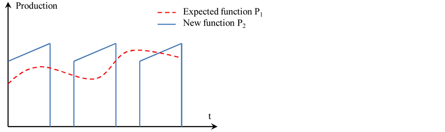
Figure 1. Construction of P2 from P1 under the constraint of averages equality.
This is a very important constraint, which leads to the smoothing and regulating the production into the intervals of productions [ti, ti + MTBF], as shown in figure 1.
For all production periods [ti, ti+1], we share the average of production P1, related to the reparation duration length (MTTR or trep), where P2 is null, on the two sides left and right as shown in figure 2. It means that we essay to have the equilibrium on the dispatching of the production quantities on all cumulus functions P2 related to the intervals [ti, ti + MTBF].
The mathematical formulation is given by equation (2).
 (2)
(2)
Or in our case, we will not adopt MTBF as a replacement time. So, we denotes the time of replacement as tr, to vary it and study the effect of its evolution on the other parameters.
In addition, we denotes the time of reparation trep and not MTTR, as we said in a previous paragraph.
equation (2) becomes:
 (2-bis)
4.2. Intervention Frequency and Maximal Capacity of Production
The frequency of intervention is considered among the most influenced parameters in maintenance policies.
The downtimes caused by systematic maintenance affect greatly the production yield, and sometimes it could be very difficult to compensate the losses by an increasing the production rate. This increasing affect directly the machines degradation state; and we try, in this paper, to study the influence of all these parameters on the choice of the coupled production and maintenance policies.
In our approach, we consider that the production horizon [t0, t0 + T] is composed by n equal periods, sum of a Time to Failure (period of good production) and Interval of Reparation.
This expression could be explained by Formula (3).
 (3)
(3)
The intervention frequency n corresponds to the integer part of the ratio of the horizon length T, by the sum of {Mean Time between Failures + Mean Time to Repair}.
In the next development, we will not consider the MTBF, and we will proceed with the periodicity of replacement, which is a variable in our case, permitting to vary the value of the reliability of the equipments.
For a reliability target, the time of replacement tr otherwise the time of good production, where P2 is not null, is given by Formula (4) in the case of Weibull low [2] .
 (4)
(4)

Figure 2. Construction de la fonction P2 entre [ti−2, ti−1].
We will also designate trep as “Time of Reparation” instead of MTTR which is constant and calculated from statistics.
By replacing the notation in Formula 4, we obtain Formula (5) expressing the intervention frequency.
 (5)
(5)
The number of interventions n permits to control the production rate and the reliability of the equipment:
• Enforcing the installations to work with a given production rate under the constraint of reliability level expected by the decision maker.
We should mention here that the concept of the reliability level is not as realistic as we think, because of the different interactions that exist between components. Weibull model and the major other statistical models used actually in the industries consider monocomponent analysis [2] .
The case of multicomponent analysis is still under study, even if the development of complex system maintenance began the 80s [3] . So the present study is interested by monocomponent system, but the developed function can be enlarged to multiplecomponents analysis and by the way find a compromise between different reliability and productivity functions. See the PhD thesis of V. Zille for more detail, in which the author grouped a large range of monocomponent and multicomponent analysis methods, and developed its own methodology to analyze this kind of problematic [4] .
This kind of compromise projects us to multicriteria optimization problems domain which could be used to resolve conflicting objectives [5] .
• A great number of interventions generate the risk that the machine will process with a high production rate to compensate the losses denoted into the maintenance interval of time; and it is clear that the production is limited by the capacity of the machines. So here is another constraint to integrate in the new production function design;
• A great number of interventions corresponds to the reduction of the periodicity tr and by the way the increasing of the reliability R. It appears clearly in the expression (3);
• Contrarily, a low frequency of interventions causes, relatively with the first configuration, higher degradation level but permits to stabilize the production during the fixed horizon. But it could generate some corrective interventions which are not taken into consideration.
So we can see here that we have two contradictory criteria and objectives; they correspond to the maximization of both reliability and production rate.
Figure 3 shows the effect of the accumulation of the production P1 on the construction of the function P2, by the effect of the downtime due to programmed maintenance interventions during a time MTTR or trep.
So, it is necessary to put a production capacity constraint (related to P2) on each period [ti, ti + tr + trep], because of the limitation of the production capacity of each machine, due to technological and logistical specifications, expressed by the production rate or maximal capacity.

Figure 3. The risk linked to capacity production exceeding.
This constraint is expressed by the equation (6).
 (6)
(6)
Where c is the nominal or the maximal production per time unit;
Remark: i is even as we will see.
5. Multiobjective Optimization Problem
After we have detailed our approach for the construction of a new production plan according to different production and maintenance constraints, we introduce, in this section, a simple mathematical formulation of the proposed problem.
The function P2 is considered linear per interval [ti, ti+1], where i is an even variable.
This function is described as follows (see figure 3):
 (7)
(7)
In this first study, we consider the same production rate (a = ai ) on all periods [ti, ti+1].
With this proposition, the parity of i, we will try to express the same reliability level on all intervals, for a fixed intervention periodicity.
Else we will obtain a serial of ai which has to be determined after by a given method. This second approach will be discussed in futures works.
Finally, the MOP [5] is defined by the following system of equations:
Maximize (R, a)
Under constraints
 (8)
(8)
 (9)
(9)
 (10)
(10)
 (4)
(4)
6. Problem Development: Characteristic Equations and Simulations
In this section, we will develop the formalism presented in the last paragraphs considering that the P1 is known from statistical estimation.
The cumulus production function P2 is considered linear and given by system of equations (7).
6.1. Production Average Equality of P1 and Cumulus Production P2 on the Production Horizon
6.1.1. Development of the Characteristic Equation
equation (8) is written:

As we mentioned, the function P1 is supposed known. So its average on [t0, t0 + T]  is known equals to “
 ”.
”.
Under the assumptions described in the system of equations (7):
• The linearity of P2 per interval [ti, ti+1] on the horizon [t0, t0 + T]
• P2 is not null on [ti, ti+1] if i is even: i = 2k
• P2 is null on [ti, ti+1] if i is odd: i = 2k + 1 (from figure 3: ti+1 = ti + trep)
P2 designates the cumulus of production, and considering the periodicity of P2, and with a variable change:
 (11)
(11)
So
 (12)
(12)
For each interval [t2k, t2k+1], and according to Figure 4, the calculation is made on the same ramp “P2(t) = at + b”, so:
 (13)
(13)
and
 (14)
(14)
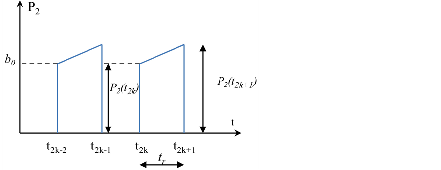
Figure 4. Measurement of P2 on [t2k, t2k+1].
equation (12) becomes:
 (15)
(15)
We obtain finally
 (16)
(16)
Remark:
The time tr expresses the systematic replacement time. So it contains the decision on the systematic maintenance policy, and it is function of the number of intervention chosen on the production horizon [t0, t0 + T].
Let’s search now the expression of the instants t2k, t2k+1 and the constants b2k.
For k varies from 0 value 1 to n ‒ 1, without much calculation, we use recursive method to express t2k and t2k+1 according to figure 3.

where t0 represents the date of the beginning of the analysis or the beginning of the production horizon having a length of T time units (hours, days…).
So the expression of the instants t2k+1 is given by equation (17):
 (17)
(17)
 (18)
(18)
Hence,
 (19)
(19)
 (20)
(20)
Let’s calculate now the value of the sum  presented on Formula (16).
Remark and some additional assumptions
• We supposed at the beginning of the paper that all the  functions, where i denotes the indices of the period [ti, ti+1] (i even), are parallel, so having the same variation a.
• Starting from equation (13), on the an interval [t2k, t2k+1], we showed that .
.
• To fix the same level of degradation on all periods, from a technical and logistical point of view in the company, we essay to have the same production levels denoted by  and
and  (figure 5):
 (21)
(21)
 (22)
(22)
According to equation (18), by replacing in equation (21):
 (23)
(23)
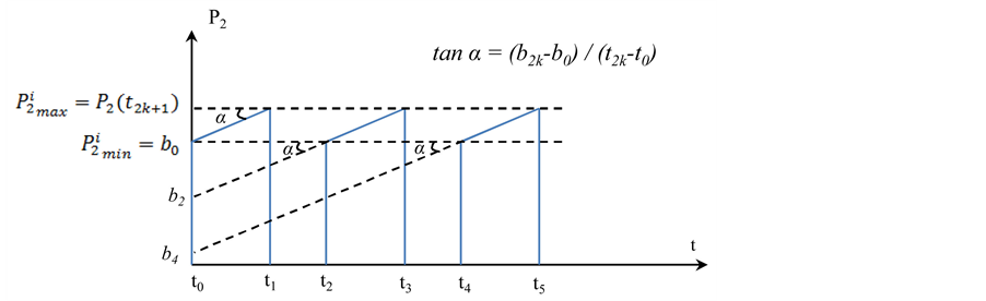
Figure 5. Representation of the b2k on the axis P2.
Let’s replace now by expressions (20) and (23) in equation (16):

 (24)
(24)
If we consider additionally t0 = 0, we find the expression of the production rate a calculated or estimated by Formula (25):
 (25)
(25)
where
 (5)
(5)
6.1.2. Characteristic Equation Analysis
We can see that equation (22) corresponds to a characteristic curve of the equality between the production average of P1 and the cumulus production P2, with the given expression of P2 by the system (7) and under the assumption of the equality of the ai.
The equation contains the principal variables which we discussed in previous sections: the productivity or the productions rate a (number of products per time unit), the interventions frequency n which can be expressed by the horizon length T, the replacement time tr and the reparation time trep.
1) Effect of the Replacement Time tr (good time of production)
Using equation (25) allows us to adjust the productivity rate a only by acting on the time of replacement, corresponding to the period of a good production. The production rate a presents hyperbolic function of the time replacement and also the intervention frequency.
We cannot analysis much more starting from the characteristic equation only, because of the complexity given by the introduction of intervention frequency n which is linked to the time replacement tr.
So we will plot the corresponding curve to see graphically the evolution of the production rate (figure 6).
2) Effect of the duration of reparation trep
In the next section, to plot an example of a = f(tr) and also the triplet (tr, a, R), we have considered a constant reparation duration trep. But it constitutes also an important variable which expresses the production downtime, and by the way to compensate the loss of production, the decider must increase the production rate a.
So it is possible to estimate the productivity, depending on the time of good production and the duration of the reparation.
3) Effect of the starting production value b0
We can also see that the first value of production at the initial instant t = t0 = 0, is very significant. It permits
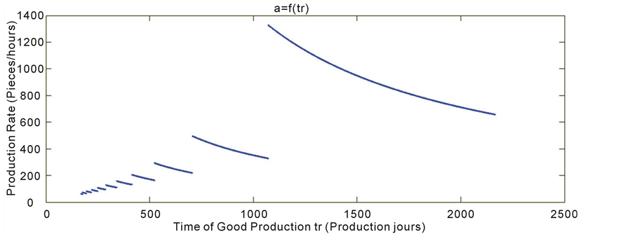
Figure 6. Production Rate a VS Replacement Time tr.
to increase or decrease the production rate, according to a big or low starting production value b0.
From a physical point of view, it is natural that if the production begins with a high value, the production velocity/rate will be less important that if the production begins with a low value. In the second case, the production rate will be as higher as possible to compensate the low starting value; this is to reach the target average of production P1.
We consider a constant time of reparation, to plot an example of the evolution of the production rate with varying tr. But it is possible to vary also the b0 and see the effect on the production rate a.
4) Relation with the reliability
Related to equation (4) and for a given degradation state which is expressed by the constants of Weibull low (γ, β, η), the variation of the reliability progresses in the inverse sense of replacement time (time of good production).
So the choice of a production and interventions policy affects directly the reliability of the corresponding equipments.
We can proceed inversely by fixing a desirable level of reliability, and calculate the time of replacement in consequence. So it will be possible to indicate the correspondent value of production rate in accordance with the desired reliability.
6.1.3. Recapitulation
After this analysis, we can conclude that by acting on the replacement time tr, time of good production, we can adjust the productivity and the reliability in the same time.
So we consider that the space of alternatives is constitutes of the different values that can take the time replacement tr to optimize the two objective functions (Reliability R, production rate a).
In the next paragraphs, we will give a numerical example to plot the resulting calculations on the function space (R, a) according to alternatives expressed by the different values of tr.
6.1.4. Simulation of the First Characteristic Equation (8) of the MOP
Actually we have just found two companies which are interested by the application of this method on their production systems.
The first progresses in generation and transportation of electricity and the other is specialized in plastic injection; and soon we will proceed to some preliminary projects to prepare the companies to have reliable information system before making any calculation or taking any decision related to our subject.
But here we will give simply an example to plot the functions and alternative space to see the evolution and the different relations between the objective functions (reliability, production rate) and the decision variable time of replacement.
1) Proposition of numerical data inputs
We are reporting here the value of the constant parameters as following:
• Systematic Reparation time trep = 24 h, corresponding to one day;
• The initial production value on the first time unit b0 = 500;
• Production horizon length T = 2190 h, corresponding to three months of continuous production;
• Estimated production average cadence on the horizon c = 15.000 pce/day;
• We vary the time of replacement from 168 h corresponding to 7 days (one week);
• A day counts 24 h of working;
2) Corresponding plots
a) Production rate a VS Replacement time tr
We report equations (25) and (5):
 (26)
(26)
where
 (5)
(5)
And

Figure 6 shows the plot, on Matlab, of the production rate a VS the Replacement Time tr witch corresponds to the time of good production.
The discontinuity of the curve is due to the introduction of the intervention frequency n which is not constant, but depends on the value of the replacement time tr.
For more comprehension, we pushed the analysis by plotting the function n = f(tr) and we obtain the graphic of figure 7.
We can see that the function “Intervention frequency n VS Replacement Time tr corresponds to a general hyperbolic behavior, which is constant “per period”.
Linked to the other terms of equation (22), we obtain the plot of Figure 6 which presents the possible values of the productivity by varying the replacement time.
b) Production Rate a VS Reliability R (Objective functions space)
As we mentioned in section 2, and in the case of reparable mechanical systems, specialists use Weibull low in order to model the reliability (or the failure occurrence) of the equipments depending on time replacement tr.
The most used models correspond to the case of mono component analysis, which does not consider any of the interactions between the components [4] .
To complete the simulation, we give an example of a machine which has a reliability function described by equation (23).
 (23)
(23)
We take: 
 ɳ = 300 h The plot of figure 8 gives the large known appearance of the exponential decreasing of the reliability according to the increasing of the time of replacement.
The 3D plot of figure 9 permits to visualize the objective functions evolution (Production Rate a and Reliability R) with the time of replacement tr (time of production) corresponding to the alternatives variable.
We have entered a production horizon of T = 365 days. In figure 6, it was a trimester T = 3 months, and that to see more the influence of the time of production on the reliability.
The plotted values constitute the feasible sets (feasible solutions and the corresponding function values) of the characteristic equation (8)

3) Conclusion of this section
Since we have found the characteristic function curve corresponding to the domain of definition of the first
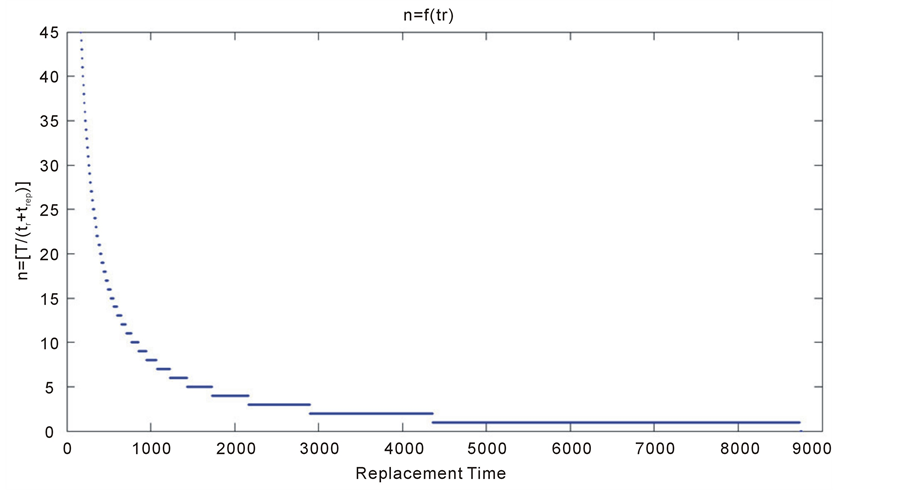
Figure 7. Intervention frequency n VS Replacement Time tr.
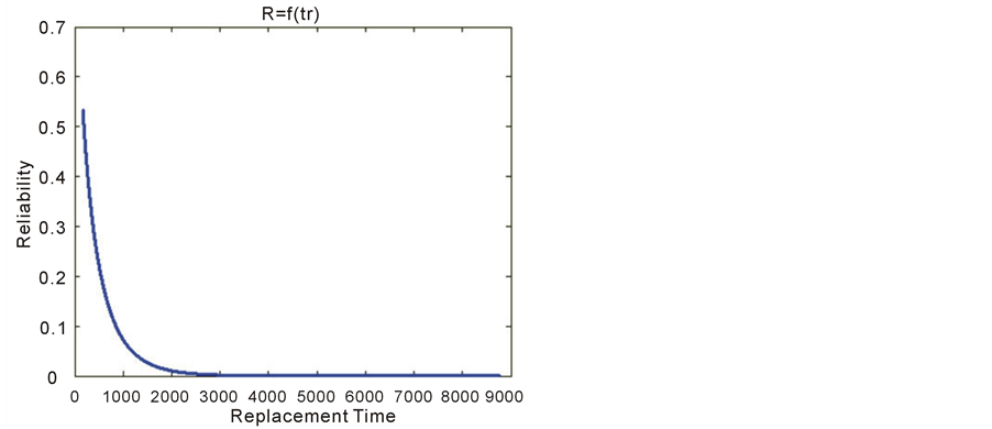
Figure 8. Reliability VS replacement time.
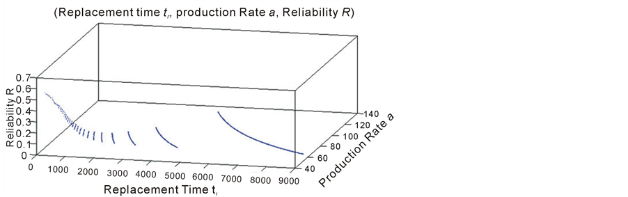
Figure 9. Plot of the triplet (Replacement time tr, production Rate a, Reliability R).
equation (8) of the MOP, defined in section 5, we will develop now the characteristic equations related to the constraints (9) and (10) defined in the MOP.
These equations permits to limit the evolution (increasing and decreasing) of the production rate a, so the constraints will limit also the corresponding feasible solutions tr, and then we will be able to present the feasible/realistic solutions of the MOP proposed to the decision makers.
6.2. Constraints on the Productivity on the Intervals [t2k, t2k+1]
6.2.1. Development of the Characteristic Equation under Maximum Capacity Constraint
In figure 3, we schematized the maximum capacity of production by a red horizontal line, which presents the risk of exceeding the higher level of production into the intervals [t2k, t2k+1].
This risk is explained by the exceeding of the capacity if the number of systematic intervention grows or decreases, and by the way, it will be necessary to fix a higher production rate a, in order to compensate the production losses.
For this reason, we put the constraints (6) in order to limit more and more the freedom of the responsible in terms of feasible realistic solutions of the triplet (tr, a, R).
This constraints constitutes the limitation for all intervals [t2k, t2k+1].
 (6)
(6)
Starting from the previous development we find the folowing equation
 (26)
(26)
Otherwise, to simplify the numerical calculations and due to the monotony of P2, we can express the equation (6) by considering only the inferiority of (P2)max compared to the maximum capacity on the interval [t2k, t2k+1]
equals to c ´ tr. And because of , we will consider following equation (27):
 (27)
(27)
According to the previous development, or by replacing in (26) the time t by the instant t2k+1, we find:
 (28)
(28)
Assuming that the function P2 is periodic, we consider the first interval of production [t0, t1] where  and k = 0.
The equation (28) becomes:
 (29)
(29)
The value on the right of equation (29) corresponds to the limitation of the production rate a.
The corresponding plot is given on figure 10.
We remark that the production limitation attains a horizontal asymptote (c = 650 pieces/hour) corresponding to the maximum of production rate given in the numerical data in the previous paragraph 6.1.4.1).
figure 11 shows the plotting of the domain definition corresponding to equation (8) of the MOP and, the limitation function (c ‒ b0/tr) corresponding to the limitation of production Rate according to equation (9) of the MOP and to figure 10.
We can see that the allure of the limitation function is near a constant value. The apparent allure is caused by the large scale of plotting which does not permit to show the evolution of the function as it is shown on figure 10.
6.2.2. Effect of the Starting Production Value b0
Figure 12 shows the effect of the variation of the starting production value b0 which is more important at low values of Replacement Time tr.
With the evolution of tr, the effect of b0 becomes neglected and the limitation function tends to the horizontal

Figure 10. Characteristic curve of the constraint (9) (P2(t) < c ´ tr).
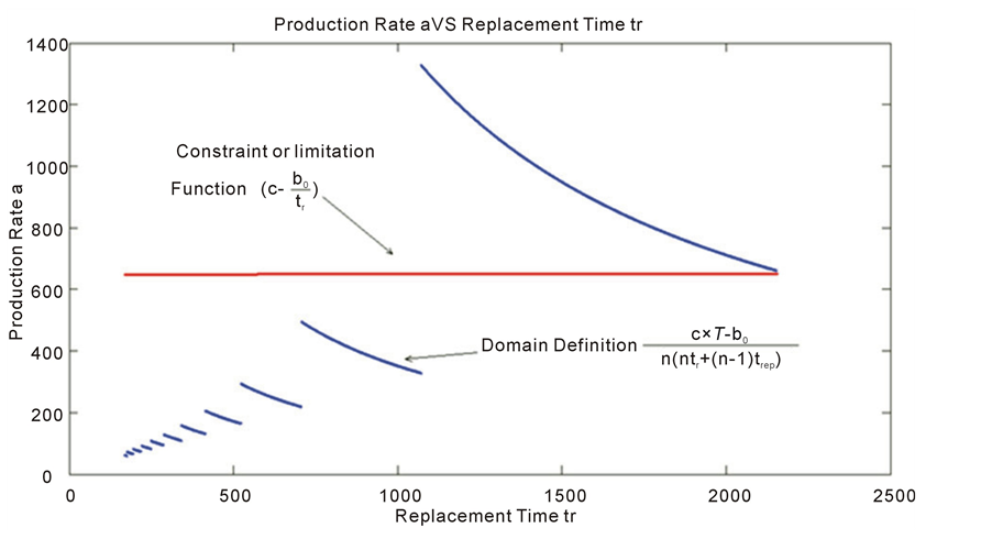
Figure 11. Feasible values of the Production Rate a (blue function) under the production constraints  (red line).
asymptote c.
We can understand this dependency by the fact that at higher Replacement Time values, the initial production b0 is not very important to reach the production average on this stage of production (cumulus).
The variables which are more important in this case are those which are linked to the reliability and the degradation state of the equipments, and also the dispersion of the process parameters variables. The variability of these parameters is affected by the robustness of the production process when the tr is on higher values.
Otherwise, at lower values of tr, the production process is more robust and can resist to the external noise, but in this case, the starting production parameters (b0 for the current study) are very important to regulate the productivity of the corresponding unit.
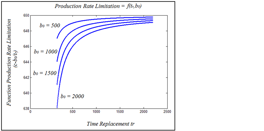
Figure 12. Production Rate a Limitation  depending on the starting production value b0.
6.2.3. Starting Production Value b0 and Equipment Reliability at Maximum Production Rate c
figure 13 shows the effect of the choice of the b0 on the corresponding Reliability value of the corresponding production equipment.
The developed expressions are made under the assumption that the starting production value b0 does not affect the reliability. Physically, it is clear that there is dependence between these two parameters: to produce b0 parts in a time ∆t we need an average production rate of b0/∆t, which affects certainly the reliability of the system.
To facilitate the analysis, the curves plotted do not consider any of these dependences.
Under the assumption made in the last previous (the independence of reliability and b0), choosing a high value of starting production b0 may reduce the production rate limitation and even the production rate a will be reduced, according to the equation (25).
It means that the reliability will evaluate in the inverse sense of b0, because the equipment will be less charged by a low value of b0, and by the way the degradation will be reduced. Reducing the degradation level is equivalent to an increasing of the corresponding reliability level.
The plot of figure 13(b) proves our supposition and shows the evolution of the couple (Production Rate Limitation, Reliability) according to the variation of b0.
6.2.4. Conclusion of This Section
After defining the first model constraint, related to equation (9) of the MOP, plotting and analyzing the corresponding allures/curves under some assumptions and according to the different maintenance and production parameters studies, let’s now see the effect of the additional constraint related to equation (10) of the MOP.
As we have seen above, the construction of the function P2 passes also by the addition of the productions, related to the downtime MTTR or trep, to the productions into the corresponding intervals [ti, ti + tr].
This information was introduced by equation (2) and expressed by equation (10) in the MOP as constraint. We have designed it by “compensation equation”.
7. Future Development and Compensation Equation: Other Model Constraint
Into the intervals [ti, ti+1] where i is even, equation (2) presents, in the left side, some terms corresponding to the production average on the intervals [ti‒1, ti+2].
Under the assumption of knowing the estimated function P1, these averages will be known by simple integral
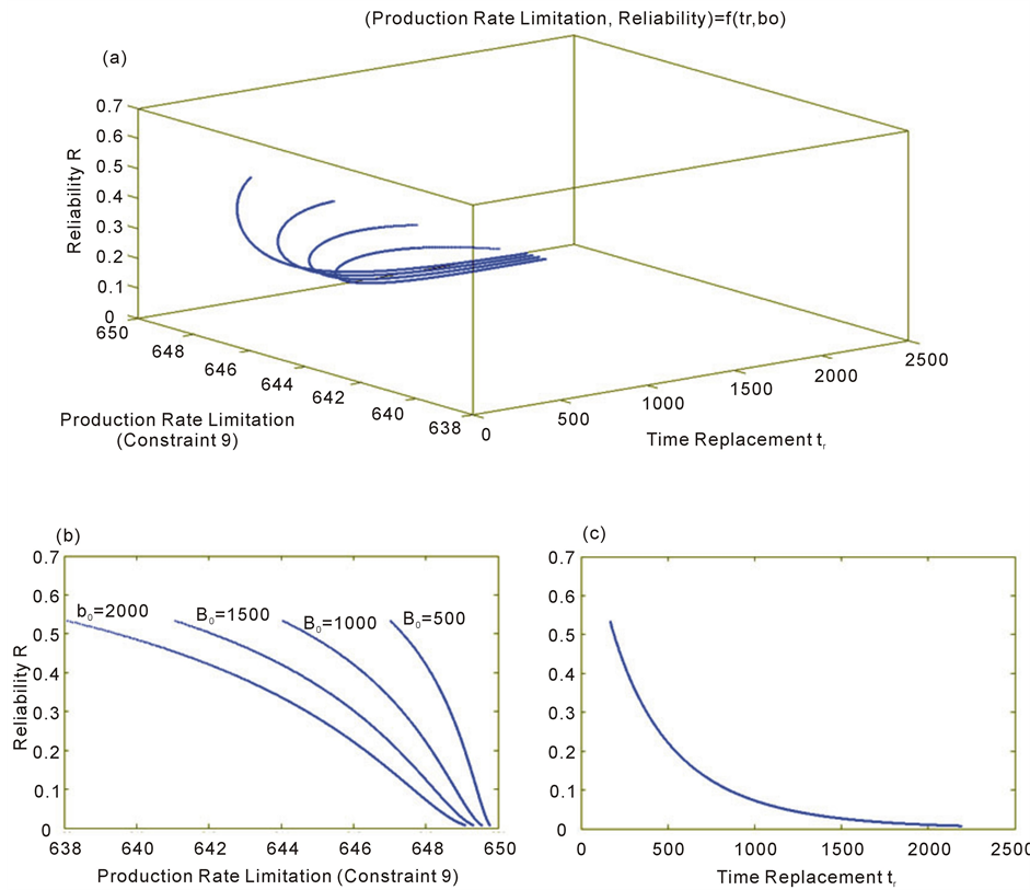
Figure 13. Plot of the production rate limitation (constraint (9)) and the reliability R depending on the replacement time tr and the starting production value b0.
calculation on any time interval.
In the next development, the constant (Cg, Cc, Cd), presented below, are supposed known. They express the averages of the expected function P1, on respectively, the intervals [ti‒1, ti], [ti, ti+1] and [ti+1, ti+2].
 (2)
(2)
i is even: i = 2k from section 6.1.a) b2k = b2k+1

and
 (18)
(18)
 (21)
(21)
We take also t0 = 0;
Hence
 (30)
(30)
We obtain finally equation (31) which expresses the minimum of production rate a which has to be fixed, in order to attain the estimated average production calculated here, per interval [t2k, t2k+1], by the constants Cl, Cc and Cr.
 (31)
(31)
In this stage we cannot make a simulation of the correspondent curve of the characterization equation (31) because we need to have sufficient information corresponding to the estimated function P1. After receiving all data, we will proceed to simulate the values of the inferior boundary of the production rate
 .
.
8. Conclusion and Perspectives
In this paper we have developed a method which permits the correction of the production plan, expressed by the estimated function P1.
The new corrected production plan P2 takes into consideration the production data, according to the estimated plan P1, the actual degradation state expressed by the constants on reliability function, and also the desired reliability level or value fixed by the responsible or imposed to the company.
The result of calculation corresponds to a set of feasible solutions, related to the choice of the systemic Replacement Time of the related to the defective parts. These feasible solutions tr gives a set of objective functions, Production Rate a and Reliability R, which are linked by the new faction P2.
So the objective is to choose production and maintenance simultaneously taking into consideration the interdependence between the two domains. The resulting set of feasible solutions will limit the degree of freedom of the company responsible in order to be as realistic as possible in the choice of the production and maintenance policies.
The correspondent simulations permitted the visualization of the functions space, which present the validity domain and the permitted choice according to the Multiobjective Optimization Problem proposed, under some assumptions and approximations.
So to summarize, the proposed methodology furnished the space definition of the production rate a, according to the expected production P1 and the equipments reliability to build the function P2, having as decision variable the time of good production denoted Replacement Time tr.
Thus, the definition domain of the production rate is obtained by this system of equation constraints:

The reliability is given by the equation:
 (23)
(23)
As perspectives, we will apply the approach on real systems, electricity production and plastics production to evaluate its validity and to make it in an advanced form.
References
- El Jai, M., et al. (2013) Integration of a Risk Analysis Method with Holonic Approach in an Isoarchic Context. International Journal of Engineering and Technology, 5, 5196-5206.
- Pocaccia, H. (2009) Introduction à l’analyse probabiliste des risques industriels in Techniques et Documentations, Lavoisier, Paris.
- Kobbacy, K.A.H. and Prabhakar Murthy, D.N. (2008) Complex System Maintenance Handbook. Springer-Verlag, London.
- Zille, V. (2009) Modélisation et évaluation des stratégies de maintenance complexes sur des systèmes multicomposants. Ph.D. Dissertation, Partnership between l’Université de Technologie de Troyes, Institut Charles Delaunay, le département Management de Risques Industriels de la division R&D d’EDF.
NOTES

*Corresponding author.