Received 31 March 2015; accepted 15 May 2015; published 18 May 2015

ABSTRACT

This paper investigates the performability of hierarchical Wireless Networked Control Systems (WNCS). The WNCS studied can operate in two modes: passive supervisor and active supervisor. It is first shown that the Markov models for both modes are identical. Performability models are then developed and a case study shows how to use these models to help make design decisions. More specifically, it is observed that the performability of a passive supervisor system increases in time while that of an active supervisor system decreases in time.

Keywords:

Performability, CTMC, Fault-Tolerance, Wireless Networked Control Systems, Hierarchical Networks, IEEE 802.11

1. Introduction

Wireless Networked Control Systems (WNCS) are a trending research topic. In Networked Control Systems (NCSs), sensors send small packets frequently to a controller. The controller processes the data in order to make decisions and forwards these decisions to the actuators [1] - [3] . Accurate timing and error-free communication are two crucial characteristics of an NCS [4] - [6] . These requirements caused CAN and PROFIBUS technologies to initially dominate the field of NCS [7] [8] . In time, evolving requirements allowed other technologies like Ethernet, PROFINET, EtherNetIP, Time-Triggered Ethernet (TT Ethernet) and Flexible TT Ethernet to gain more widespread use in NCSs [7] [9] - [12] .

The move to WNCS solutions has been a trend due to the freedom, robustness and simplicity offered by wireless alternatives. WNCS facilitate installation and decrease maintenance costs [13] [14] . One commercially available WNCS system is Wireless Interface for Sensors and Actuators [13] . A similar system was also introduced in [14] . The system in [14] had 30 sensors and 30 actuators connected through Wi-Fi to two Access Points (APs). The Access Points (APs) are connected through switched Ethernet to a controller [11] [14] [15] . Both systems in [13] and [14] were able to fulfill the delay requirements with zero packets drops.

In [16] , the model in [14] was improved to allow for the concatenation of three cells. The model fulfilled the delay conditions in the presence of interference with fault-tolerance on the controller level. A performability [17] analysis was done to assess the robustness of the system in [16] .

In [18] , hierarchical fault-tolerance was applied to the system in [16] by adding a supervisor above the controller level. The supervisor has two modes of operation: either active or passive. In the active mode, the supervisor intervenes immediately if a controller fails. In the passive mode, another operational controller takes over the functions of the failed controller; the supervisor intervenes only if all controllers fail. The difference in modes required different data flow models.

In this paper the performability of the active and passive modes in [18] will be compared. Markov reliability models will be built for both systems. Then a reward will be assigned to each state in the system. A case study will demonstrate the use of the model as a design tool to help make appropriate design choices regarding active and passive supervisor modes.

The rest of the paper is divided as follows: Section 2 summarizes the work on the wireless workcells and performability analysis. Section 3 presents the Markov model for the active and passive modes while Section 4 presents the performability model. A case study is carried out in Section 5 based on the proposed performability models. Section 6 concludes the work done.

2. Background

A WNCS model is described in [14] . In this model, the workcell has 30 sensors and 30 actuators communicating over unmodified IEEE 802.11b with two APs. The APs are connected to the controller through switched Ethernet. Sensors send their data to the controller. The controller processes the data gathered from the sensors and communicates the needed actions to the actuators [14] . The delay between sensors sending their data and decisions arriving at the actuator should meet a certain deadline. UDP is used as the transport layer for all types of communication within the workcell. The workcell dimensions are 3 m × 3 m [14] .

In order to improve system operation, the study in [16] replaced IEEE 802.11b with IEEE 802.11g as IEEE 802.11g provides more bandwidth. Consequently, only one AP was needed to operate the workcell. Hence, concatenating three cells became achievable with three non-interfering channels. In the concatenated system, each sensor sends three copies of each sample to the three controllers, but only the designated controller responds. When a controller fails, another controller is assigned to take over its functions. The network was able to meet the delay deadlines with zero packet loss with only one working controller and in the presence of interference. The delay varied depending on the number of operational controllers. The system was considered more robust when the difference between the measured delay and the benchmark delay was bigger. Transient performability [17] was then used to evaluate the robustness of the three concatenated cells. As a first step, a reliability model was built using a Continuous Time Markov Chain (CTMC). Next, each state of the Markov model was assigned a reward. The reward for a state was calculated as the difference between the average end-to-end delay, in that state, and the maximum allowable delay. The rationale behind choosing this reward is that the difference between the system deadline and the maximum observed end-to-end delay is an indication of the robustness of the system.

In [18] , a supervisor was added to the three-workcell system in [16] as shown in Figure 1. The supervisor can handle the control of the cells in two ways: passive or active. In the passive mode, the supervisor handles the control functions only if all controllers fail. In the active mode, once a controller fails, the supervisor takes over its control tasks. Multicasting was used in [18] to decrease the load on the wireless network. Multicasting allowed each sensor to send only one stream of packets to the AP. The AP duplicates the stream as needed and forwards it to the designated controllers through switched Ethernet. In passive supervisor systems, the AP sends four copies of the packet stream over the wired backbone, one to each controller and another to the supervisor. In active supervisor systems, only two copies of the packet stream are sent over the wired backbone, one to the designated controller and another to the supervisor. Duplication of streams is needed to provide for seamless control take over in case of failure. The data load on the network differs from the passive mode to the active supervisor mode; hence, the experienced end-to-end delays differ.

3. Markov Model

Figure 2 shows the Markov model representing the operation of the fault-tolerant architecture described above. It consists of five states. Next is an explanation of each of the five states as well as the transitions between these states. The system starts in State {3K + S}. This is the starting state where the system is in the fault-free condition and the three controllers (K) as well as the supervisor (S) are fully operational. It was assumed in [18] that the supervisor is extremely reliable and will fail last. Consequently, if any of the three controllers fail, the system moves to State {2K + S}. Assuming that the time to failure is exponentially distributed [19] , the rate of this transition is 3λ_k where λ_k is the failure rate of any of the three controllers (it is assumed that the three controllers are identical and therefore have the same failure rate λ_k). Note that the Mean Time to Failure (MTTF) is equal to (1/λ_k). The system moves back to State {3K + S} with a rate of µ_k where µ_k is the repair rate of any of the three controllers (it is assumed that the three controllers are identical and therefore have the same repair rate µ_k). The repair time is also assumed to have an exponential distribution and the Mean Time To Repair (MTTR) is equal to (1/µ_k) [19] .

From State {2K + S}, the system moves to State {1K + S}. This indicates that a second controller has failed before the first failed controller was repaired. The rate of this transition is 2λ_k since any of the two remaining controllers could fail. The transition back from State {1K + S} to State {2K + S} is equal to 2µ_k with the assumption that 2 repair persons are available [19] . With one controller operational, the system moves to State {0K + S} at a rate λ_k. In this state, all three controllers have failed and the supervisor is carrying out the entire control task [18] . If any of the three failed controllers is repaired before the failure of the supervisor, the system moves back to State {1K + S} at a rate of 3µ_k (assuming three repair persons).

If the supervisor fails while the system is in State {0K + S}, the entire system fails and goes to State {F}. Remember that it was assumed in [18] that the supervisor fails last because of its relatively high reliability compared to that of the controllers. The transition rate between States {0K + S} and {F} is λ_s which is the failure rate of the supervisor. In State {F}, the entire production line has failed. It will be assumed that management will

wait until all faults are repaired to take the system back to its fully operational State {3K + S}. The rate of this transition is µ_sys.

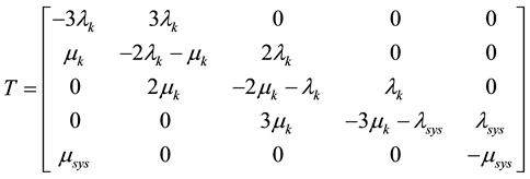
For simplicity, let states {3K + S}, {2K + S}, {1K + S}, {S} and {F} be represented as states 4, 3, 2, 1 and 0. Let be the probability of residing in state i (i = 4, 3, 2, 1, 0) at time t. Let T be the Transition Rate Matrix. The transient probability of residing in any of the five states can be calculated using the following Chapman­ Kolmogorov equations as follows [19] :

(1)

(2)

(3)

(4)

(5)

(6)

(7)

(8)

Also, and. The Chapman­Kolmogorov equations can be solved to obtain P_i(t) for i = 4, 3, 2, 1, 0.

4. Reward and Performability

Performability is an important metric to assess the robustness of a fault-tolerant system [17] . It simultaneously takes into account component failures and performance. Performability starts with a Markov model (like the one depicted in Figure 2) and assigns a reward (or penalty) to each state. In this paper, the same strategy as in [16] will be followed. The reward will be equal to the difference between the system end-to-end delay in any state and the deadline. Obviously, the higher this difference, the higher the system robustness and performance. The delays were measured with OPNET with a 95% confidence analysis. Table 1 shows the upper bounds of the confidence interval for the end-to-end delays of the system under study in the passive mode while Table 2 shows the same values for the active mode. As the delay approaches the 36 ms benchmark, the packets experience a higher risk of missing the allowable deadline.

It is important to note that some states can be associated with several delay values. For example, State {2K + S} indicates that one controller has failed. Six different scenarios are possible: Controller i fails and either Controller j or Controller k takes over its tasks (i, j, k = 1, 2, 3 and i ≠ j ≠ k ≠ 0). Some of these scenarios have identical delays because of symmetry such as the failure of Controller 1 with Controller 2 taking over and vice-versa (with maximum end-to-end delay = 7.26 ms in the passive mode). The highest delay among the six scenarios will be used to calculate the reward for State {2K + S} to obtain the worst-case performability.

The Transient Performability TP(t) is calculated as follows [17] :

(9)

where R_i is the reward associated with State i.

5. Case Study

A case study was carried out, based on the methodology outlined in Section 3, in order to compare between the performability of the active and passive supervisor modes for the hierarchical WNCS proposed in [18] . SHARPE [20] was used in order to carry out the performability analysis based on the Markov model illustrated in Figure 2 and the values for the reward per state for each of the passive and active modes as in Table 1 and Table 2 respectively. The employed failure rates λ_k and λ_s were 1 month∙s⁻¹ and 0.25 month∙s⁻¹ respectively as the supervisor is assumed to be more robust than the controllers. Also, the employed repair rates µ_k and µ_sys

were 2 month∙s⁻¹ and 1 month∙s⁻¹ respectively as the repair time is expected to be larger when repairing the entire system after the failure of the supervisor. Figure 3 illustrates the resulting performability curves over time for both the active and passive supervisor modes.

5.1. Passive Supervisor

Based on Equation (9), the Transient Probability (TP) is calculated as the summation of the result of multiplying the probability of residing in a state by the reward of the state. The reward (R) is the difference between the benchmark and the delay. The delay is calculated as the maximum end-to-end delay between the sensors and actuators using a 95% confidence analysis.

In the first state {3K + S}, where all controllers are functional, the end-end delay is 9.33 ms. In the second state {2K + S} when one controller fails, six options are available: either controller 1 or 2 or 3 fails and one of the functioning controllers would take over. As per [18] , failures of the first and third controller have same delays due to symmetry. Moreover, failure of controller 1 with controller 2 taking over has same delays as controller 2 failing with controller 1 taking over. This leaves two distinctive options for state {2K + S}; either controller 1 failing and controller 2 taking over or controller 1 failing and controller 3 taking over. The higher of the two delays was the delay of the state where controller 1 failed which was 7.26 ms. For the third state {K + S}, the combinations available after eliminating symmetrical options would be either failure of controller 1 and controller 2 or failure of controller 1 and 3. Controller 3 and controller 1 failure had the higher delay of 8.6ms. In the final state, when all controllers fail {S} only one value of the delay is available of 8.73ms. The highest possible delay of each state in passive supervisor scenario is shown in Table 1.

From Figure 3, it can be seen that the performability of the passive supervisor mode is at its lowest at t = 0. In other words, the fault-free state is where the passive supervisor mode has the worst performance. This is due to the fact that, for the passive mode, the data transmitted from the sensors belonging to the three cells is quadrupled over the wired backbone (once to each of the three controllers and again to the supervisor). As such, the experienced overall packet end-to-end delays are higher than in the faulty scenarios with do not require as much packet duplication. The observed perfomability of the passive supervisor mode stabilizes over time to around 27.53 ms.

5.2. Active Supervisor

The delays for the active supervisor states are calculated the same way as delays in passive supervisor. Symme- trical cases are eliminated to leave the following states: All controller functional in {3K + S}, failure of controller

1 or controller 2 with the supervisor taking over to represent state {2K + S}, and failure of controllers 1 and 2 or 1 and 3 to represent the {K + S} state and all controllers fail in state {S}. The highest delay of each state is chosen to represent the delay of the state and shown in Table 2. The same values for were used as in the passive supervisor performability analysis. The curve for TP(t) was drawn based on the active reward shown in Table 2.

From Figure 3, it can be noticed that the performability of the active supervisor mode is at its highest at t = 0. Thus, the active mode offers the best performance during the fault-free state. As controllers start to fail, all traffic is rerouted to the supervisor node which becomes responsible for the control of all failed cells. The added network delays result in an increase in overall packet end-to-end delay and consequently lower performance. The observed performability of the active supervisor mode stabilizes over time to around 28.65 ms.

6. Conclusions

Wired control systems are replaced by Wireless Networked Control Systems in factory automation due to robustness and flexibility offered by the wireless option. Wireless workcell communication for factory automation was proposed in previous literature. The workcell had 30 sensors and 30 actuators communicating wirelessly through IEEE 802.11 to an Access Point (AP). The AP is connected to a controller through switched Ethernet protocol. Hierarchical fault-tolerance was added to the system in order to add a supervisor to a three-workcell system. The supervisor could either be passive or active. If the supervisor was active, the supervisor would take over functions of any controller once it fails. However, if the supervisor was passive, the supervisor would intervene only if all controllers failed.

This paper has compared the performability of passive and active supervisor systems. As a first step, the Markov model of both systems was built. It was shown that the Markov model is the same for both situations. The model had five states: all controllers and supervisor functioning, two controllers and supervisor functioning, one controller and supervisor functioning, only the supervisor functioning, and then total system failure state. The failure rate of the supervisor was considered much less than failure rate of a controller as it was considered to be more robust than the controllers. However, the repair rate of the full system when supervisor fails is considered to be much higher than the repair rate of a single controller.

The transient probabilities for each system were calculated through summing the probabilities of residing in each state multiplied by the reward of each state. The reward was considered as the difference between the highest possible end-to-end delay on each state and the benchmark of 36 ms. As the difference increases, the system is considered more robust, as the probability of a packet exceeding the benchmark decreases.

A case study was carried out based on the aforementioned methodology in order to compare the performability of a hierarchical passive and active supervisor WNCS. It was shown that the performability of a passive supervisor system improves over time while that of an active supervisor system degrades over time. However, the active supervisor mode was shown to consistently offer higher performability compared to the passive mode over time.

References

- Skeie, T., Johannessen, S. and Brunner, C. (2002) Ethernet in Substation Automation. IEEE Control Systems, 22, 43-51. http://dx.doi.org/10.1109/MCS.2002.1003998
- Nilsson, J. (1998) Real-Time Control Systems with Delays. PhD Thesis, Department of Automatic Control, Lund Institute of Technology, Lund.
- Lian, F.L., Moyne, J.R. and Tilbury, D.M. (2001) Networked Control Systems Toolkit: A Simulation Package for Analysis and Design of Control Systems with Network Communication. Technical Report UM-ME-01-04. http://www.eecs.umich.edu
- Daoud, R.M., ElSayed, H.M., Amer, H.H. and Eid, S.Z. (2003) Performance of Fast and Gigabit Ethernet in Networked Control Systems. Proceedings of the IEEE Midwest Symposium on Circuits and Systems MWSCAS, Cairo, 27-30 December 2003, 505-508. http://dx.doi.org/10.1109/MWSCAS.2003.1562328
- Felser, M. (2005) Real-Time Ethernet Industry Prospective. Proceedings of the IEEE, 93, 1118-1129. http://dx.doi.org/10.1109/JPROC.2005.849720
- Decotignie, J.D. (2005) Ethernet-Based Real-Time and Industrial Communications. Proceedings of the IEEE, 93, 1102-1117. http://dx.doi.org/10.1109/JPROC.2005.849721
- Official Site for PROFIBUS and PROFINET. http://www.profibus.com
- Bosch (1991) CAN Specification Version 2.0, ISO 11898.
- EtherNet/IP Adaptation of CIP Specification (2001). http://read.pudn.com/downloads166/ebook/763212/EIP-CIP-V2-1.0.pdf
- International Electrotechnical Commission. IEC 61784-1 and 61784-2. www.iec.ch
- IEEE 802.3 Standard.
- Pedreiras, P., Almeida, L. and Gai, P. (2002) The FTT-Ethernet Protocol: Merging Flexibility, Timeliness and Efficiency. Proceedings of the IEEE Euromicro Conference on Real-Time Systems ECRTS, Vienna, 19-21 June 2002, 134- 142.
- Steigmann, R. and Endresen, J. (2006) Introduction to WISA: WISA―Wireless Interface for Sensors and Actuators. White Paper, ABB.
- Refaat, T.K., Daoud, R.M., Amer, H.H. and Makled, E.A. (2010) WiFi Implementation of Wireless Networked Control Systems. Proceedings of the 7th IEEE International Conference on Networked Sensing Systems INSS, Kassel, 15-18 June 2010, 145-148. http://dx.doi.org/10.1109/INSS.2010.5573993
- IEEE 802.11 Standard.
- Refaat, T.K., Daoud, R.M. and Amer, H.H. (2012) Fault-Tolerant Controllers in Wireless Networked Control System Using 802.11g. Proceedings of the IEEE International Conference on Industrial Technology ICIT, Athens, 19-21 March 2012, 783-788. http://dx.doi.org/10.1109/ICIT.2012.6210034
- Haverkort, B.R., Marie, R., Rubino, G. and Trivedi, K. (2001) Performability Modelling: Techniques and Tools. John Wiley & Sons, Hoboken.
- Makled, E.A, Halawa, H.H., Daoud, R.M., Amer, H.H. and Refaat, T.K. (2015) WiFi-Based Hierarchical Wireless Networked Control Systems. Proceedings of the IEEE International Conference on Industrial Technology ICIT, Seville, 17-19 March 2015, 1964-1969.
- Siewiorek, D.P. and Swarz, R.S. (1998) Reliable Computer Systems―Design an Evaluation. A. K. Peters, Natick.
- Official Site for SHARPE. http://sharpe.pratt.duke.edu/