Intelligent Control and Automation
Vol. 3 No. 4 (2012) , Article ID: 24859 , 10 pages DOI:10.4236/ica.2012.34035
Application of Current Search to Optimum PIDA Controller Design
Department of Electrical Engineering, South-East Asia University, Bangkok, Thailand
Email: deachap@sau.ac.th
Received August 8, 2012; revised September 8, 2012; accepted September 15, 2012
Keywords: Current Search; Metaheuristics; PIDA Controller; AVR System
ABSTRACT
An application of the current search (CS), one of the most efficient metaheuristic optimization search techniques, to design the PIDA (proportional-integral-derivative-accelerated) controllers is proposed in this paper. The CS is applied to search for the optimum PIDA controller’s parameters. The obtained controllers are tested against nine benchmark systems collected by Åsström and Hägglund considered as the hard-to-be-controlled plants and an automatic voltage regulator (AVR) system. As results, the optimum PIDA controllers can be successfully obtained by the CS and the responses of controlled systems are very satisfactory.
1. Introduction
Since the PID (proportional-integral-derivative) controller was proposed by Minorsky in 1922 [1], the PID family (PI, PD, and PID) has been a worldwide solution for an effective control. It has been played the most important role as the heart of control engineering practice for many years [2]. However, in some particular situations, PID controllers are not suitable especially for higherorder control systems. In 1996, the PIDA (proportionalintegral-derivative-accelerated) controller was introduced by Jung and Dorf [3], and claimed to deliver faster and smoother response as well as more suitable for the higher-order plants than the PID could. The PIDA controller has been successfully applied to torsional resonance suppression [4], and induction motor control [5], [6], respectively. However, the conventional design of the PIDA controller proposed by Jung and Dorf [3] based on the dominant pole concept does not govern the complex plants [6].
To date, metaheuristic optimization has become potential candidates and widely applied to various engineering problems. Over five decades, many efficient metaheuristics have been developed for combinatorial and continuous optimization problems and they have been applied to many successful real-world applications [7]. By literatures, several metaheuristic techniques, i.e., evolutionary programming (EP) [8], tabu search (TS) [9], simulated annealing (SA) [10], genetic algorithm (GA) [11], ant colony optimization (ACO) [12], particle swarm optimization (PSO) [13], harmony search (HS) [14], bacterial foraging optimization (BFO) [15], shuffled frog leaping algorithm (SFLA) [16], bee colony optimization (BCO) [17], key cutting search (KCS) [18], firefly search (FS) [19], hunting search (HuS) [20], cuckoo search (CuS) [21], and current search (CS) [22] etc., have been consecutively launched. These algorithms can be classified into different groups depending on their nature of criteria being considered, such as natural-inspired population based and single-solution based. Among single-solution based optimization approaches, the current search (CS) is one of the latest metaheuristics proposed in 2012 [22]. It has been also successfully applied to design the PID controllers for unstable systems [23]. In 2010, the optimum PIDA controller design by the GA has been introduced [6]. Although the GA is efficient to find the global minimum, it consumes too much search time. Thus, the CS is expected to be an alternative potential algorithm to obtain optimum PIDA controllers. In this paper, the CS algorithm is briefly reviewed and then applied to design optimum PIDA controllers for nine benchmark systems collected by Åström and Hägglund [24] and an automatic voltage regulator (AVR) system [25]. This paper consists of six sections. The problem formulation of PIDA design is described in Section 2. A brief of the CS algorithm is provided in Section 3. The CS-based PIDA design for benchmark systems is illustrated in Section 4. Application of the CS to optimum PIDA design for the AVR system is described in Section 5, while the conclusions are given in Section 6.
2. Problem Formulation
According to the classical control context, a conventional control loop is represented by the block diagram in Figure 1. The PIDA controller receives the error signal,  , and produces the control signal, U(s), to control and regulate the output response,
  , referred to the reference input, R(s), while D(s) is an external disturbance signal, Gp(s) and Gc(s) are the plant and the controller transfer functions, respectively.
The transfer function of the PIDA controller is expressed in Equation (1), where Kp, Ki, Kd, and Ka are the proportional, integral, derivative, and accelerated gains, respectively, while d, e, and f are filter parameters. An alternative representation in a polynomial form results in Equation (2) with the following parameters: Kp, Ki, Kd, Ka, a, and b, respectively. The design objective is to achieve a minimum response error due to a unit step input. Hence, the following performance specifications i.e. rise time, percent overshoot, settling time, and steadystate errors, are considered.
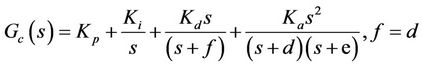 (1)
(1)
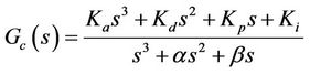 (2)
(2)
The block diagram in Figure 2 represents the use of the CS to design the PIDA controllers. The objective function, J, the sum of absolute errors between R(s) and C(s) as stated in Equation (3), is fed back to the CS tuning block. J is minimized to find the optimum PIDA controller’s parameters giving satisfactory responses.
 (3)
(3)
3. Current Search (CS) Algorithm
The current search (CS) is one of the most efficient metaheuristic optimization search techniques. The CS
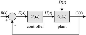
Figure 1. Conventional control loop.
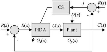
Figure 2. CS-based PIDA design.
algorithm is inspired by an electric current flowing through electric networks [22]. Algorithms of the CS are briefly described step-by-step as follows.
Step 1. Initialize the search space W, iteration counter k = j = 1, maximum allowance of solution cycling jmax, number of initial solutions (feasible directions of currents in network) N, number of neighborhood members n, search radius r, and set Y = G = X = Æ.
Step 2. Uniformly random initial solution Xi, i = 1, ···, N within W. Evaluate the objective function  of "X. Rank Xi, i = 1, ···, N giving
 , then store ranked Xi into set Y.
Step 3. Let x0 = Xk as selected initial solution.
Step 4. Uniformly random neighborhood xi, i = 1, ···, n around x0 within radius r. Evaluate the objective function  of "x. A solution giving the minimum objective function is set as x*.
Step 5. If , keep x0 in set Gk and set x0 = x*, set j = 1 and return to Step 4. Otherwise update j = j + 1.
Step 6. If j < jmax, return to Step 4. Otherwise keep x0 in set X and update k = k + 1.
Step 7. Stop the search process when termination criteria (TC) are satisfied. The optimum solution found is x0. Otherwise return to Step 3.
The diagram in Figure 3 reveals the search process of the CS algorithm. The search space W in Step 1 is performed as the feasible boundary where the electric current can flow. The maximum allowance of solution cycling jmax implies the local entrapment occurred in the selected direction. The number of initial solutions N is set as feasible directions of the electric currents in network. The number of neighborhood members n is provided as the sub-directions of the electric currents in the selected direction, and the search radius r is given as the sub-search space where the electric current can flow in the selected direction.
The uniformly random approach is conducted in Step 2 to perform the feasible directions of the electric currents. These directions will be ranked by the objective function to arrange the signification of directions from most to least. Once the most significant direction of the current is selected in Steps 3-5, the search process will consecutively find the optimum solution along the most significant direction within the sub-search space where the electric current can flow in the selected direction. Each feasible solution will be evaluated via the objective function until the optimum solution is found. In Steps 6 and 7, the local entrapment in the selected direction will be identified via the maximum allowance of solution cycling. If occurred, the second, the third, and so on, of the significant direction ranked in Step 2 will consecutively employed, until optimum solution will be found or the TC will be met.

Figure 3. Flow diagram of the CS algorithm.
Another search technique among single-solution based optimization approaches is tabu search (TS) [9]. For algorithm comparison, the CS differs from the TS in that the CS possesses several distributed directions ranked beyond the search space to be searched so far, while the TS starts the search process at any random initial solution. Although the TS has the tabu list used to record the visited solution and avoid the process visits the prohibited (tabu) area, diversification and intensification of solution finding of the CS are superior to the TS.
4. PIDA Design for Benchmark Systems
The CS-based PIDA controller design for benchmark systems is described in this section. Referring to Figure 2, the parameter tuning process is repeatedly performed to minimize the objective function J stated in (4) until the TC is met. In this work, the maximum search round countmax = 200 is set as the TC. The number of initial solutions N = 10 is set as feasible directions. The number of neighborhood members n = 20 and the search radius r = 1% of search space are priory set.
 (4)
(4)
To perform the performance of the proposed design method, the CS is applied to design the PIDA controllers for nine benchmark systems collected by Åström and Hägglund [24] as summarized in Table 1. These systems are considered as a class of hard-to-be-controlled plants to design the PIDA controllers by conventional design methods or tuning rules. The objective function J with the performance specification constraints in Equation (4) will be minimized by the CS, where tr is rise time, P.O. is percent overshoot, ts is settling time, and ess is steady state error. The objective function J in Equation (4) consisting of time-domain response specifications (first four inequality constraints) is used as the strategy to evaluate the system performance in control context. The ranges of the controller parameters are bounded by lower and upper values to be searched. These are set as the inequality constraints of the optimization problem as also stated in Equation (4). The numeric values of design specifications and ranges of the parameters are summarized in Tables 2 and 3, respectively.
In this work, the CS algorithm was coded by MATLAB running on Intel Core2 Duo 2.0 GHz 3 Gbytes DDR-RAM computer. The tests were conducted 100 trial runs against each plant to obtain the best solution found. As obtained results, the step input and the step disturbance responses are depicted in Figures 4-12. Figure 13 shows the convergence rate curves of the objective function J of the Plant 1 as an example. The convergence rate curves of other plants are omitted because they have a similar form to those in Figure 13. The optimum PIDA controllers resulted from the CS-based method and the numerical results concerning performances are summa-
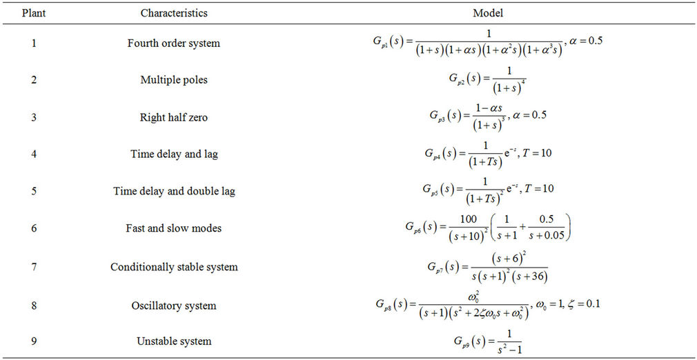
Table 1. Plant models and characteristics.
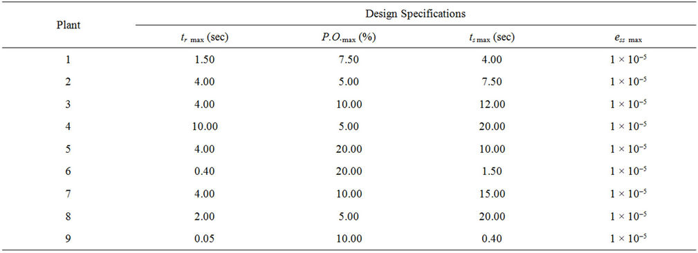
Table 2. Design specifications.
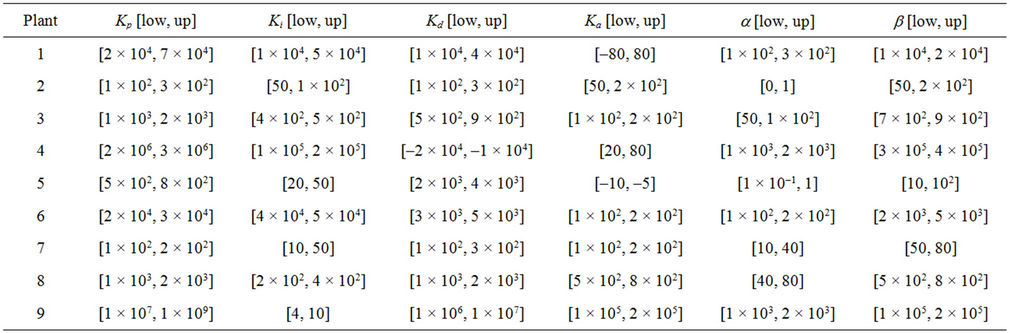
Table 3. Range of the PIDA controller parameters.

Figure 4. Step responses of Plant 1.

Figure 5. Step responses of Plant 2.
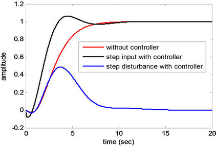
Figure 6. Step responses of Plant 3.
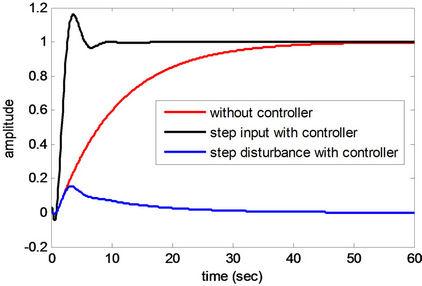
Figure 7. Step responses of Plant 4.
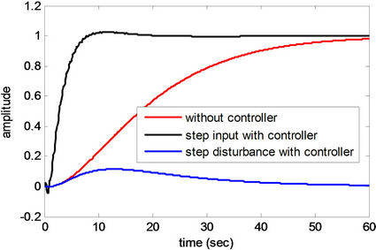
Figure 8. Step responses of Plant 5.

Figure 9. Step responses of Plant 6.
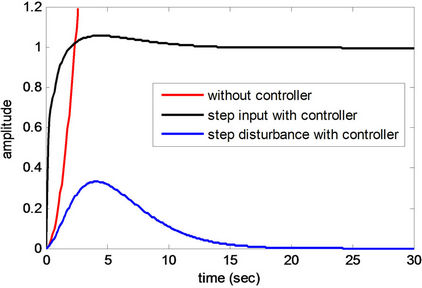
Figure 10. Step responses of Plant 7.
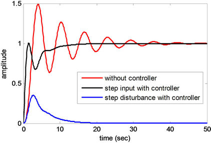
Figure 11. Step responses of Plant 8.
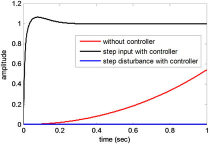
Figure 12. Step responses of Plant 9.
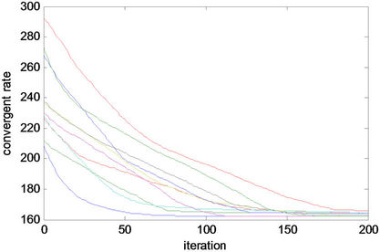
Figure 13. Convergent curves of Plant 1.
rized in Tables 4 and 5, respectively. In case of the Plant 1, for example, the optimum PIDA controller can be successfully optimized. The CS results Kp = 5.1 × 10⁴, Ki = 3.13 × 10⁴, Kd = 2.1 × 10⁴, Ka = –50.4, a = 250, and b = 1.9 × 10⁴ with 7.7041 × 10² sec. of search time consumed. The step input response of the controlled system gives tr = 1.23 sec., P.O. = 5.68%, ts = 3.34 sec., and ess = 0.0, while the step disturbance response of the controlled system yields tre = 6.37 sec. and P.O. = 26.76%.
From Figures 4-12 and Tables 4 and 5, obtained results confirm that all controlled systems with the PIDA controllers optimized by the CS satisfactory respond to the input commands in terms of rapid settling, low overshoot, and stabilization, and rapidly recover from the external disturbances. It can be noticed that the optimum PIDA controllers obtained from the CS-based method well perform both command-following (tracking) and disturbance rejections (regulating) objectives.
5. PIDA Design for AVR System
An automatic voltage regulator (AVR) is commonly used in the generator excitation system of hydro and thermal power plants to regulate generator voltage and control the reactive power flow [25]. The main role of the AVR is to hold the terminal voltage of a synchronous generator
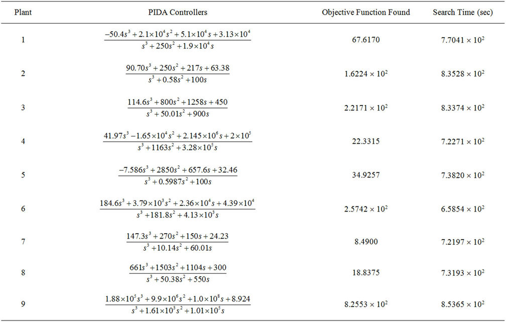
Table 4. Optimum PIDA controllers.
at a specified level. A synchronous generator connecting to power system would critically affect the security of the power system depending on the stability of the AVR.
A simple AVR consists of four main components, i.e. amplifier, exciter, generator, and sensor, respectively. A simplified AVR system controlled by the PIDA controller is represented by the block diagram in Figure 14, where Ve is the error voltage between the reference input voltage Vref (s) and sensor voltage, while Vu , Vr, and Vf are the controlled, amplified, and excited voltage signals, and V(s) is the output voltage.
In Figure 14, four main components of the AVR are linearized and modeled by transfer functions [25] as follows.
• Amplifier model The amplifier model is expressed in Equation (5) by a gain KA and a time constant tA. Typical values of KA are in the range of 10 to 400. The amplifier time constant is very small ranging from 0.02 to 0.1 sec. [25]. In this work, KA = 10 and a time constant tA = 0.1 sec. are priory set.
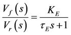
• Exciter model The exciter model is stated in Equation (6) by a gain KE and a time constant tE. Commonly values of KE are in the range of 1 to 400 and the time constant tE is from 0.25 to 1.0 sec. [25]. In this work, KE = 1 and a time constant tE = 0.4 sec. are priory assumed.
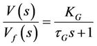
• Generator model The generator model is linearized and expressed in Equation (7). A gain KG may vary between 0.7 to 1.0, and the time constant tG between 1.0 to 2.0 sec. [25]. In this work, we assumed KG = 1 and a time constant tG = 1 sec. are set as a priory.
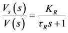
• Sensor model The generator model is a simple firstorder transfer function as stated in Equation (8) with a gain KR, and the time constant tR ranging from of 0.001 to 0.06 sec. [25]. In this work, KR = 1 and tR = 0.01 sec. are assumed.
 (5)
(5)
 (6)
(6)
 (7)
(7)
 (8)
(8)
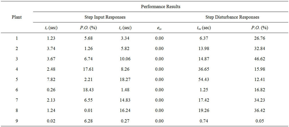
Table 5. Performance results.
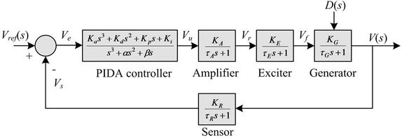
Figure 14. Closed loop AVR system with PIDA controller.
 (9)
(9)
Figure 15 shows the original terminal voltage step response of the AVR system without the PIDA controller. Uncontrolled system provides tr = 0.2639 sec., P.O. = 50.61%, ts = 6.9834 sec., and ess = 0.0909, respectively.
Referring to Figure 2, the CS-based PIDA controller design is conducted for the AVR system. The objective function J, sum of absolute errors between  and
and , will be minimized according to inequality constraints in Equation (9). The maximum search round countmax = 200 is set as the TC. N = 10, n = 20, and r = 1% of search space are priory set. In this application, the genetic algorithm (GA) and the tabu search (TS) are also conducted to compare there effectiveness. In Figure 2, the CS block will be replaced by GA and TS, respectively. For a fair comparison, the parameter settings are set as follows: For GA, number of population = 200, crossover rate = 40%, mutation rate = 10%, and uniformly random approach is conducted; For TS, number of neighborhood members = 200, search radius = 10% of search space, aspiration criteria are employed, and uniformly random approach is also conducted. Both GA and TS use the maximum search round countmax = 200 as the TC. Algorithms of GA, TS, and CS were coded by
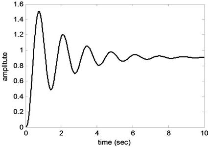
Figure 15. Step response of AVR system without PIDA controller.
MATLAB running on Intel Core2 Duo 2.0 GHz 3 Gbytes DDR-RAM computer. The tests were conducted 50 trial runs for each technique to obtain the optimum PIDA controller.
The step input and the step disturbance responses of controlled AVR systems are depicted in Figure 16. As results, it was found that the optimum PIDA controller can be successfully achieved by GA, TS, and CS according to inequality constraints stated in Equation (9). However, the responses of the AVR system with the PIDA controller optimized by the CS are superior to others in terms of least overshoot and fastest settling time. In details, the PIDA controller optimized by the GA results Kp = 784.0012, Ki = 342.1474, Kd = 577.5625, Ka = 99.1016, a = 592.9654, and b = 912.4471 with 198.4501 sec. of search time consumed. The step input response (red-solid line in Figure 16) gives tr = 0.4512 sec., P.O. = 6.01%, ts = 2.5422 sec., and ess = 0.0, while the step disturbance response (red-dashed line in Figure 16) provides tre = 4.1522 sec. and P.O. = 19.06%. Then, the PIDA controller optimized by the TS gives Kp = 824.8747, Ki = 341.6321, Kd = 592.3258, Ka = 102.2365, a = 596.1974, and b = 854.1247 with 122.6642 sec. of search time consumed. The step input response (bluesolid line in Figure 16) results tr = 0.4128 sec., P.O. = 8.24%, ts = 2.5687 sec., and ess = 0.0, while the step disturbance response (blue-dashed line in Figure 16) gives tre = 4.1498 sec. and P.O. = 19.05%. Finally, the PIDA controller optimized by the CS results Kp = 799.1201, Ki = 394.0112, Kd = 498.9516, Ka = 101.0102, a = 589. 5411, and b = 965.0501 with 104.4465 sec. of search time consumed. The controlled system provides very satisfactory step responses with tr = 0.5248 sec., P.O. = 1.82%, ts = 1.3406 sec., ess = 0.00 for command following (black-solid line in Figure 16) and tre = 4.1541 sec., P.O. = 19.07% for disturbance rejections (black-dashed line in Figure 16). It can be noticed again that the optimum PIDA controller can be successfully obtained from the CS. The designed AVR system with PIDA controller

Figure 16. Step responses of AVR system with PIDA controller.
optimized by the CS can provide very satisfactory responses better than the GA and TS in terms of smoothest and fastest response.
6. Conclusion
Obtaining an optimum PIDA controller via the current search (CS) has been proposed in this paper. As one of the most efficient metaheuristic optimization search techniques, the CS is flexible and suitable for various optimization problems in which control synthesis application is one of the domains. In this paper, the CS algorithm has been briefly reviewed. The CS has been applied to obtain optimum PIDA controllers against nine systems proposed by Åström and Hägglund and an automatic voltage regulator (AVR) system for benchmarking. As contributions of this work, the optimum PIDA controllers can be successfully obtained by the CS for all systems giving very satisfactory tracking and regulating responses.
REFERENCES
- N. Minorsky, “Directional Stability of Automatically Steered Bodies,” American Society of Naval Engineering, Vol. 34, No. 2, 1922, p. 284.
- A. Dwyer, “Handbook of PI and PID Controller Tuning Rules,” Imperial College Press, London, 2003. doi:10.1142/p277
- S. Jung and R.C. Dorf, “Analytic PIDA Controller Design Technique for a Third Order System,” Proceedings of the 35th IEEE Conference on Decision and Control, Kobe, 11-13 December 1996, pp. 2513-2518.
- C. U. Thaiwasin, S. Sujitjorn, Y. Prempraneerach and J. Ngamwiwit, “Torsional Resonance Suppression via PIDA Controller,” Proceedings of the IEEE Region 10 Conference TENCON, Kuala Lumpur, Vol. 3, 2000, pp. 498- 503.
- D.-Y. Ha, I.-Y. Lee, Y.-S. Cho, Y.-D. Lim and B.-K. Choi, “The Design of PIDA Controller with Pre-Compensator,” Proceedings of the IEEE International Symposium on ISIE, Pusan, Vol. 2, 2001, pp. 798-804.
- S. Sornmuang and S. Sujitjorn, “GA-Based PIDA Control Design Optimization with an Application to AC Motor Speed Control,” International Journal of Mathematics and Computers in Simulation, Vol. 4, No. 3, 2010, pp. 67- 80.
- D. T. Pham and D. Karaboga, “Intelligent Optimisation Techniques,” Springer, London, 2000. doi:10.1007/978-1-4471-0721-7
- L. J. Fogel, A. J. Owens and M. J. Walsh, “Artificial Intelligence through Simulated Evolution,” John Wiley, Hoboken, 1966.
- F. Glover and M. Laguna, “Tabu Search,” Kluwer Academic Publishers, Dordrecht, 1997. doi:10.1007/978-1-4615-6089-0
- S. Kirkpatrick, C. D. Gelatt and M. P. Vecchi, “Optimization by Simulated Annealing,” Science, Vol. 220, No. 4598, 1983, pp. 671-680. doi:10.1126/science.220.4598.671
- D. E. Goldberg, “Genetic Algorithms in Search Optimization and Machine Learning,” Addison Wesley Publishers, Edmonton, 1989.
- M. Dorigo, “Optimization, Learning and Natural Algorithms,” PhD Thesis, Politecnico di Milano, 1992.
- J. Kennedy and R. Eberhart, “Particle Swarm Optimization,” Proceedings of the IEEE International Conference on Neural Networks, Vol. 4, 1995, pp. 1942-1948. doi:10.1109/ICNN.1995.488968
- Z. W. Geem, J. H. Kim and G. V. Loganathan, “A New Heuristic Optimization Algorithm: Harmony Search,” Simulation, Vol. 76, No. 2, 2001, pp. 60-68. doi:10.1177/003754970107600201
- K. M. Passino, “Biomimicry of Bacterial Foraging for Distributed Optimization and Control,” IEEE Control System Magazine, Vol. 22, No. 3, 2002, pp. 52-67. doi:10.1109/MCS.2002.1004010
- M. M. Eusuff and K. E. Lansey, “Optimization of Water Distribution Network Design Using the Shuffled Frog Leaping Algorithm,” Journal of Water Resource Planning and Management, Vol. 129, No. 3, 2003, pp. 210- 225. doi:10.1061/(ASCE)0733-9496(2003)129:3(210)
- D. T. Pham, A. Ghanbarzadeh, E. Koç, S. Otri, S. Rahim and M. Zaidi, “The Bees Algorithm—A Novel Tool for Complex Optimisation Problems,” Proceedings of the IPROMS Conference, 2006, pp. 454-461.
- J. Qin, “A New Optimization Algorithm and Its Application—Key Cutting Algorithm,” Grey Systems and Intelligent Services, Nanjing, 10-12 November 2009, pp. 1537-1541.
- X. S. Yang, “Firefly Algorithms for Multimodal Optimization, Stochastic Algorithms,” Foundations and Applications SAGA 2009, Lecture Notes in Computer Sciences, Vol. 5792, 2009, pp. 169-178. doi:10.1007/978-3-642-04944-6_14
- R. Oftadeh, M. J. Mahjoob and M. Shariatpanahi, “A Novel Mata-Heuristic Optimization Algorithm Inspired by Group Hunting of Animals: Hunting Search,” Computers and Mathematics with Applications, Vol. 60, No. 1, 2010, pp. 2087-2098. doi:10.1016/j.camwa.2010.07.049
- X. S. Yang and S. Deb, “Engineering Optimization by Cuckoo Search,” International Journal of Mathematical Modeling and Numerical Optimization, Vol. 1, No. 4, 2010, pp. 330-343. doi:10.1504/IJMMNO.2010.035430
- A. Sukulin and D. Puangdownreong, “A Novel MetaHeuristic Optimization Algorithm: Current Search,” Proceedings of the 11th WSEAS International Conference on Artificial Intelligence, Knowledge Engineering and Data Bases (AIKED’ 12), Cambridge, 22-24 February 2012, pp. 125-130.
- D. Puangdownreong and A. Sukulin, “Obtaining an Optimum PID Controllers for Unstable Systems Using Current Search,” International Journal of Systems Engineering, Applications & Development, Vol. 6, No. 2, 2012, pp. 188-195.
- K. J. Åström and T. Hägglund, “Benchmark Systems for PID Control,” IFAC Digital Control: Past, Present and Future of PID Control, Terrassa, 5-7 April 2000, pp. 165- 166.
- Z. L. Gaing, “A Particle Swarm Optimization Approach for Optimum Design of PID Controller in AVR System,” IEEE Transactions on Energy Conversion, Vol. 19, No. 2, 2004, pp. 384-391. doi:10.1109/TEC.2003.821821