Journal of Information Security
Vol.5 No.3(2014), Article
ID:47876,23
pages
DOI:10.4236/jis.2014.53010
Parallelized Hashing via j-Lanes and j-Pointers Tree Modes, with Applications to SHA-256
Shay Gueron1,2
1Department of Mathematics, University of Haifa, Haifa, Israel
2Intel Corporation, Israel Development Center, Haifa, Israel
Email: shay@math.haifa.ac.il
Copyright © 2014 by author and Scientific Research Publishing Inc.
This work is licensed under the Creative Commons Attribution International License (CC BY).
http://creativecommons.org/licenses/by/4.0/


Received 1 May 2014; revised 1 June 2014; accepted 28 June 2014
ABSTRACT
j-lanes tree hashing is a tree mode that splits an input message into j slices, computes j independent digests of each slice, and outputs the hash value of their concatenation. j-pointers tree hashing is a similar tree mode that receives, as input, j pointers to j messages (or slices of a single message), computes their digests and outputs the hash value of their concatenation. Such modes expose parallelization opportunities in a hashing process that is otherwise serial by nature. As a result, they have a performance advantage on modern processor architectures. This paper provides precise specifications for these hashing modes, proposes appropriate IVs, and demonstrates their performance on the latest processors. Our hope is that it would be useful for standardization of these modes.
Keywords:Tree Mode Hashing, SHA-256, SIMD Architecture, Advanced Vector Extensions Architectures, AVX, AVX2

1. Introduction
This paper expands upon the j-lanes tree hashing mode which was proposed in [1] . It provides specifications, enhancements, and an updated performance analysis. The purpose is to suggest such modes for standardization. Although the specification is general, we focus on j-lanes tree hashing with SHA-256 [2] as the underlying hash function.
The j-lanes mode is a particular form of tree hashing, which is optimized for contemporary architectures of modern processors that have SIMD (Single Instruction Multiple Data) instructions. Currently deployed SIMD architectures use either 128-bit (e.g., SSE, AVX [3] , NEON [4] ) or 256-bit (AVX2 [3] ) registers. For SHA-256, an algorithm that (by its definition) operates on 32-bit words, AVX and AVX2 architectures can process 4 or 8 “lanes” in parallel, respectively. The j-lanes mode capitalizes on this parallelization capability.
The AVX2 architecture [3] includes all the necessary instructions to implement SHA-256 operations efficiently: 32-bit shift (vpsrld) and add (vpaddd), bitwise logical operations (vpandn, vpand, vpxor), and the 32-bit rotation (by combining two shifts (vpsrld/vpslld) with a single xor/or (vpxor) operation).
The future AVX512f instructions set [3] [5] supports 512-bit registers, ready for operating on 16 lanes. It also adds a few useful instructions that would increase the parallelized hashing performance: rotation (vprold) and ternary-logic operation (vpternlogd). The (vpternlogd) instruction allows software to use a single instruction for implementing logical functions such as Majority and Choose, which SHA-256 (and other hash algorithms) use. Rotation (vprold) can perform the SHA-256 rotations faster than the vpsrld + vpslld + vpxor combination.
2. Preliminaries
Hereafter, we focus on hash functions (HASH) that use the Merkle-Damgård construction (SHA-256, SHA-512, SHA-1 are particular examples). Other constructions can be handled similarly. Suppose that HASH produces a digest of d bits, from an input message M whose length is length (M). The hashing process starts from an initial state, of size i bits, called an Initialization Vector (denoted HashIV). The message is first padded with a fixed string plus the encoded length of the message. The resulting (padded) message is then viewed and processed as the concatenation M||padding = m0||m1||…||mk−1 of k consecutive fixed size blocks m0m1...mk−1.
The output digest is computed by an iterative invocation of a compression function compress (H, BLOCK). The inputs to the compression function are a chaining variable (H) of i bits, and a block (BLOCK) of b bits. Its output is an i-bit value that can be used as the input to the next iteration. The output digest (of HASH) is f(Hk−1). We call an invocation of the compression function an “Update” (because it updates the chaining variable).
We use here the following notations:
Ÿ ⌈x⌉: floor(x).
Ÿ ⌊x⌋: ceil(x) = floor(x + 1).
Ÿ S[y: x]: bits x through y of S.
Ÿ ||: string concatenation (e.g., 04||08 = 0408).
Ÿ HASH: the underlying hash function; HASH = HASH (message, length (message)).
Ÿ HashIV the Initialization Vector used for HASH (e.g., for SHA-256 Hash IV = 0x6a09e667, 0xbb67ae85, 0x3c6ef372, 0xa54ff53a, 0x510e527f, 0x9b05688c, 0x1f83d9ab, 0x5be0cd19; when written as 8 integers).
Ÿ compress (H, BLOCK): the compression function used by HASH. It consumes a single fixed sized data chunk (BLOCK) of the message, a state (H), and updates H (at output) according to a specified algorithm ([2] defines the compression function for SHA-256).
Ÿ M: the hashed message.
Ÿ N: the length, in bits, of M.
Ÿ L: the length, in bytes, of M (L = [N/8]).
Ÿ d: the length, in bits, of the digest that HASH produces.
Ÿ D: the length, in bytes, of the digest that HASH produces (D = [d/8]).
Ÿ B: the length, in bytes, of the message block consumed by the compression function compress (e.g., for SHA-256, B = 64).
Ÿ j: the number of lanes used by the j-lanes hashing process (in this paper, we discuss only j = 4, 8, 16).
Ÿ Q: the size, in bits, of the “word” that HASH uses during the computations (Q = 32 for SHA-256, and Q = 64 for SHA-512).
Ÿ W: the size, in bytes, of the “word” that HASH uses during the computations (W = Q/8).
Ÿ S: the number of lanes that a given architecture supports, with respect to the word size of HASH (e.g., AVX architecture has registers (xmm’s) that can hold 128 bits. For HASH = SHA-256, Q = 32, therefore, S = 128/Q = 4).
Ÿ P: the length, in bytes, of the minimal padding length of HASH (for SHA-256, a bit “1” is concatenated, and then the message bit length (N), encoded as an 8-byte Big Endian integer. Therefore, with SHA-256, we have P = 9).
3. The j-Lanes Tree Hash
The j-lanes tree hash is defined in the context of the underlying hash function HASH, and j (j ≥ 2) is a parameter. We are interested here in j = 4, 8, 16. The input to the j-lanes hash function is a message M whose length is N bits.
This message is (logically) divided into k (k ≥ 0) consecutive Q-bit “words” mi, i = 0, 1, …, k − 1 (if M is the NULL message, then k = 0).
When k ≥ 1, the words mj, j = 0, 1, …, k − 2 (if k − 2 < 0, there are no words in the count) consist of Q bits each. If N is not divisible by Q, then the last word mk−1 is incomplete, and consists of only (N mod Q) bits.
We then split the original message M into the j disjoint sub-messages (buffers) Buff0, Buff1, …, Buffj−1 as follows:
Buff0 = m0||mj||mj×2 …
Buff1 = m1||mj+1||mj×2+1 …
...
Buffj−1 = mj−1||mj×2−1||mj×3−1 …
Note if N ≤ Q × (j − 1), then one or more buffers Buffi will be a NULL buffer. If N = 0 all the buffers are defined to be NULL, and will be hashed as the empty message (i.e. only the padding pattern is hashed in that case).
After the message is split into j disjoint buffers, as described above, the underlying hash function, HASH, is independently applied to each buffer as follows:
H0 = HASH (Buff0, length (Buff0))
H1 = HASH (Buff1, length (Buff1))
H2 = HASH (Buff2, length (Buff2))
…
Hj−1 = HASH (Buffj−1, length (Buffj−1))
The j-lanes digest (H) is defined by H = DIGEST (HASH, M, length (M), j) = HASH (H0||H1||H2||…||Hj−1, j × D)
Remark 1: The final stage of the process is called the wrapping stage. It hashes a message with a fixed size of j × D bytes. The number of updates required is ⌈(j×D+P)/B⌉ that are likely to be serial updates.
Remark 2: The API for a j-lanes hash for a fixed j would be the same as for the underlying hash, i.e. for SHA-256, the j-lanes implementation could have the following API: SHA256_j_lanes (uint8_t* hash, uint8_t* msg, size_tlen).
Example 1: Consider a message M with N = 4096 bits, and the hash function HASH = SHA-256 that operates on 32-bit words (Q = 32). Here, k = ⌈4096/32⌉ = 128. For j = 8 we get Buff0 = m0||m8||m16 …||m120
Buff1 = m1||m9||m17 …||m121
Buff2 = m2||m10||m18 …||m122
Buff3 = m3||m11||m19 …||m123
Buff4 = m4||m12||m20 …||m124
Buff5 = m5||m13||m21 …||m125
Buff6 = m6||m14||m22 …||m126
Buff7 = m7||m15||m23 …||m127
where each one of the eight buffers is 512 bit long.
Example 2: Consider a message M with N = 2913 bits, and HASH = SHA-256 (Q = 32). Here, k = ⌈2913/32⌉ = 92. Since 2913 mod 32 = 1, the last word, m91, consists of only a single bit. For j = 8, we get Buff0 = m0||m8||m16 …||m80||m88
Buff1 = m1||m9||m17 …||m81||m89
Buff2 = m2||m10||m18 …||m82||m90
Buff3 = m3||m11||m19 …||m83||m91
Buff4 = m4||m12||m20 …||m84
Buff5 = m5||m13||m21 …||m85
Buff6 = m6||m14||m22 …||m86
Buff7 = m7||m15||m23 …||m87
Here, |Buff0| = |Buff1|=|Buff2| = 384 bits, |Buff3| = 353 bits, |Buff4| = |Buff5| = |Buff6| = |Buff7| = 352 bits.
Example 3: Consider a message M with N = 100 bits, and HASH = SHA-256 (Q = 32). Here, k = ⌈100/32⌉ = 4. Since 100 mod 32 = 4, the last word, m3, consists of only 4 bits. For j = 8, we get Buff0 = m0
Buff1 = m1
Buff2 = m2
Buff3 = m3
Buff4 = NULL Buff5 = NULL Buff6 = NULL Buff7 = NULL
Here, |Buff0| = |Buff1| = |Buff2|=32 bits, |Buff3| = 4 bits, |Buff4| = |Buff5| = |Buff6| = |Buff7| = 0 bits.
Remark 3: Similarly to the serial hashing, the j-lanes hashing can process the message incrementally (e.g., when the messages is streamed). Since the parallelized compression operates (in parallel) on consecutive blocks of j × B bytes, it needs to receive only the “next j × B bytes” in order to compute an Update.
4. The j-Pointers Tree Hash
An alternative way to define j “slices” of the message M, is to provide j pointers to j disjoint buffers Buff0, ..., Buffj−1, of M, together with k values for the length of each buffer. In this case, it is also required that Ʃi length (Buffi) = length (M).
In this case, the j-pointers tree hash procedure would be the following. Compute the j hash values for each of the disjoint buffers:
H0 = HASH (Buff0, length (Buff0))
H1 = HASH (Buff1, length (Buff1))
H2 = HASH (Buff2, length (Buff2))
...
Hj−1 = HASH (Buffj−1, length (Buffj−1))
Produce the output digest H = HASH (H0||H1||H2||…||Hj−1, j × D)
Remark 4: In a software implementation, the API of the j-lanes function is the same as the API for any other hash function (see Remark 2).The function computes the buffers and their length internally. On the other hand, the API to a j-pointers hash requires a pointer to each buffer and its length, to be provided by the caller. For example:
SHA256_4_pointers(uint8_t* hash, uint8_t* buff0, size_tlen0, uint8_t* buff1, size_tlen1, uint8_t* buff2, size_tlen2, uint8_t* buff3, size_tlen3)
or, alternatively:
SHA256_j_pointers(uint8_t* hash, uint8_t** buffs, size_t*lengths, unsigned int j)
5. The Difference between j-Pointers Tree Hash and j-Lanes Tree Hash
The j-pointers and the j-lanes tree modes are essentially the same construction, and the difference is in how the message is viewed (logically) as j slices. The j-lanes tree mode has a performance advantage when implemented on SIMD architectures because it supports natural sequential loads into the SIMD registers: each word is naturally placed in the correct lane (see Figure 1).
The j-pointers tree mode expects the data to be loaded from j locations. It is more suitable for implementations on multi-processor platforms, and for hashing multiple independent messages into a single digest (e.g., hashing a complete file-system while keeping a single digest). Of course, a j-pointers tree can also be used on a SIMD architecture, but in that case it requires “transposing” the data in order to place the words in the correct position in the registers. This (small) overhead is saved by using the j-lanes tree mode.
6. Counting the Number of Updates
The performance of a standard (serial) hash function is closely proportional to the number of Updates (U) that the computations involve, namely
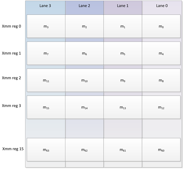
Figure 1. The j-lanes tree mode natural data alignment with SIMD architectures (here, with 128-bit registers (xmm’a) as 4 32-bit words).
![]() (1)
(1)
In Equation (1), each Update consumes B additional bytes of the (padded) message, and the number of bytes in the padded message is at least L + P (with no more than a single block added by the padding).
For the j-lanes hash (with the underlying function HASH), the number of serially computed Updates can be approximated by
 (2)
(2)
Note that some of the j-lanes Updates are carried out in parallel, compressing min(S, j) blocks per one Update call. Equation (2) accounts for parallelizing at most min(S, j) block compressions, thus contributing the term ⌈L/(min(j,S) × B)⌉, plus one Update for the padding block. A padding block is counted for each lane, although, depending on the length of the message, some Updates are redundant. The wrapping step cannot be parallelized (in general) and adds ⌈(j × D + P)/B⌉ serial Updates to the count.
Example 4: Suppose that HASH = SHA-256, and consider a message of 1024 bytes. The standard SHA-256 function requires ⌈(1024 + 9)/64⌉ = 17 Updates. We compare this to the count of j-lanes Updates for a few values of j:
For the AVX2 architecture (Haswell architecture [3] ) we have D = 32, B = 64, P = 9, S = 8. This implies that the 8-lanes SHA-256 (j = 8) is optimal. It requires ⌈1024/(8 × 64)⌉ + 1 + ⌈(8 × 32 + 9)/64⌉ = 8 Updates.
For the AVX architecture (Sandy Bridge architecture), we have S = 4, so, j = 4 is the optimal choice for this setup, and the 4-lanes SHA-256 (j = 4) requires ⌈1024/(4 × 64)⌉ + 1 + ⌈(4 × 32 + 9)/64⌉ = 8 Updates. Of course, it is possible to use the 8-lanes SHA-256 on this architecture, but we can only parallelize 4 Updates using the xmm registers. Therefore, the 8-lanes SHA-256 (j = 8) on the AVX architecture (where S = 4) requires ⌈1024/(4 × 64)⌉ + 1 + ⌈(8 × 32 + 9)/6⌉ = 10 Updates.
Figures 2-4 show the number of Update calls (some are parallelized). As seen on Figure 2, when the number of lanes is limited by the SIMD architecture, the total number of Updates for the different choices of j, varies only by the number of Updates that are required by the final wrapping stage.
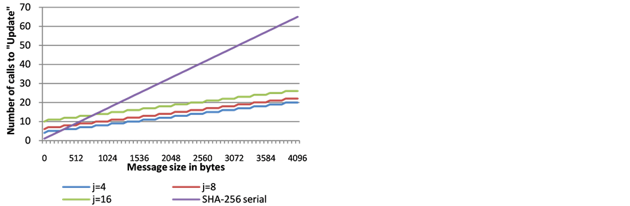
Figure 2. The number of serially computed Updates required on a SIMD architecture supporting 4 lanes (e.g., AVX on a Sandy Bridge architecture), for different message lengths and different choices of j.
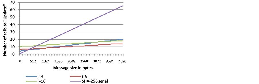
Figure 3. The number of serially computed Updates required on a SIMD architecture supporting 8 lanes (e.g., AVX2 on a Haswell architecture), for different message lengths and different choices of j.
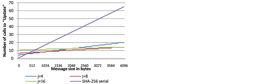
Figure 4. The number of serially computed Updates required on a SIMD architecture supporting 16 lanes (AVX512f —a future architecture), for different message lengths and different choices of j.
However, in Figure 4, we see the differences when the choice of j = 16 becomes the most efficient for message sizes of 4 KB and up, requiring the fewest Updates. For 4 KB messages, both j = 16 and j = 8 require 14 Updates, j = 4 requires 20 updates and the serial SHA-256 requires 65 Updates.
7. The j-Lanes Hash and the j-Pointers Hash with Different IVs
The Merkle-Damgård construction uses one d-bit IV to initialize the computations. For j-lanes hashing, one might prefer to modify the IVs and this section proposes a method to achieve that.
Define j + 1 “Prefix” blocks (“Pre”) as follows:
 (3)
(3)
where
Ÿ j is encoded as a 32-bit integer in little-endian notation.
Ÿ i in the “index” of the lane, and is encoded as a 32-bit integer in little-endian notation. The values i = 0, …, j − 1 are used for the lanes, and the value i = j is used for the wrapping step.
Ÿ type is a single byte with the value 0x0 for a j-lanes hash, and 0x1 for a j-pointers hash.
Ÿ HASH is the name of the underlying hash function, encoded as a string of ASCII characters. For SHA-256 we write HASH = “SHA256” or, as ASCII, 0x53, 0x48, 0x41, 0x32, 0x35, 0x36 (encoding “S” = 0x53, “H” = 0x48, “A” = 0x41 etc.).
Ÿ The number of characters (NCHAR) in the string that indicates HASH should be such that NCHAR + 9 ≤ B.
The Prefix blocks are prepended to the j + 1 hashed messages, and modify the “effective” IV that is being used. In other words, the j-lanes algorithm executes the following computations:
H0 = HASH (Pre0||Buff0, length (Buff0) + B)
H1 = HASH (Pre1||Buff1, length (Buff1) + B)
H2 = HASH (Pre2||Buff2, length (Buff2) + B)
...
Hj−1=HASH (Prej-1||Buffj-1, length (Buffj−1) + B)
H = HASH (Prej||H0||…||Hj−1, j × D + B)
Remark 5: SHA-256 allows hashing a message of any length less than 264 bits. In the j-lanes/j-pointers modes, the length of the message should be less than 264 − 512 bits.
Pre-Computing the IVs
The Prefix blocks do not need to be re-computed for each message. Instead, the j + 1 IV values can be precomputed by:
 (4)
(4)
Note that the Prefix blocks can also be viewed as a modification of HASH, to use the new IVs instead of a fixed IV. For convenience, denote the hash function that uses IVi by HASH’i. In that case the SHA-256 padding shall still accommodate the length of the prefix block.
With this notation, the j-lanes hashing can be expressed in terms of HASH’ by:
H0 = HASH’0 (Buff0, length (Buff0))
H1 = HASH’1 (Buff1, length (Buff1))
H2 = HASH’2 (Buff2, length (Buff2))
...
Hj−1 = HASH’j−1 (Buffj−1, length (Buffj−1))
H = HASH’j (H0||H1||H2||…||Hj−1, j × D)
Figure 5 shows the values of the prefix blocks and the new IVs (for HASH = SHA-256).
Remark 5: the following alternative can be considered, for saving the space of storing j + 1 IV values. Instead, use a single (new) IV value for all the j + 1 hash computations. We fixed one value of idx, namely idx = j + 1, and define the j-lanes hash by:
H0 = HASH’j+1(Buff0, length (Buff0))
H1 = HASH’j+1(Buff1, length (Buff1))
...
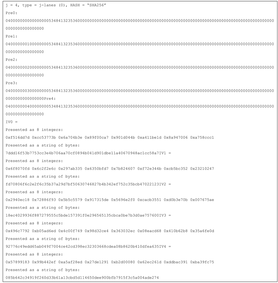
Figure 5. An example for the Prefix blocks and the IVs generation for the 4-lanes SHA-256 hash function.
Hj−1 = HASH’j+1(Buffj−1, length (Buffj−1))
H = HASH’j+1(H0||H1||H2||…||Hj−1, j × D)
Figure 6 shows the values of the prefix block and the new IV (for HASH = SHA-256) for the alternative.
Test vectors for j-lanes SHA-256 with j = 4, 8, 16 are provided in the Appendix.
8. Performance
This section shows the measured performance of j-lanes SHA-256, for j = 4, 8, 16, and compares it to the performance of the serial implementation of SHA-256. The results are shown in Figure 7 and Figure 8.
Clearly, the j-lanes SHA-256 has a significant performance advantage over the serial SHA-256, for messages that are at least a few kilobytes long. The choice of j affects the hashing efficiency: for a given architecture, j-lanes SHA-256 with j > S is slower than j-lanes SHA-256 with the optimal choice of j = S, due to the longer wrapping step. However, the differences become almost negligible for long messages.
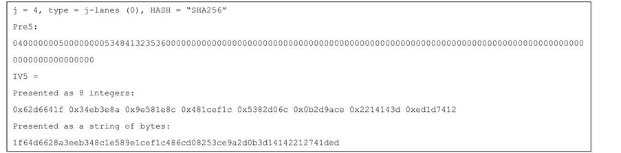
Figure 6. An example of the Prefix block and the (single) IV generation, for the 4-lanes, SHA-256 hash function, for the variant that uses only one modified IV.
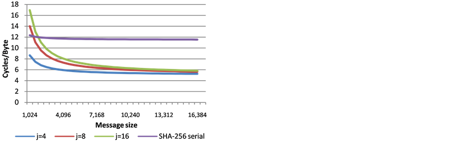
Figure 7. Performance of SHA-256 j-lanes compared to the serial SHA-256 implementation, Intel Architecture Codename Sandy Bridge (S = 4).
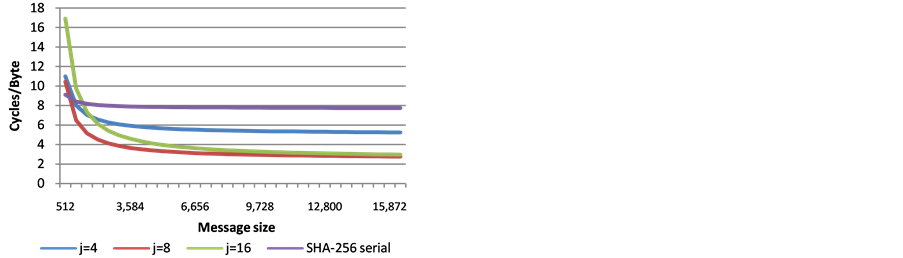
Figure 8. Performance of SHA-256 j-lanes compared to the serial SHA-256 implementation, Intel Architecture Codename Haswell (S = 8).
9. Conclusions
This paper showed the advantages of a j-lanes hashing method on modern processors, and provided information on how it can be easily defined and standardized.
The choice of j is a point that needs discussion. If a standard supports different j values, then the optimal choice can be selected per platform. This, however, could add an interoperability burden, and we can imagine that a single value of j would be preferable. In this context, we point out that Figure 2 and Figure 3 (theoretical approximations) are consistent with Figure 7 and Figure 8 for j = 4 and j = 8 (actual measurements). Therefore, Figure 4 can be viewed as a good indication for what can be expected when using j = 16 on the future architectures that would introduce the AVX512f architecture (supporting S = 16). Furthermore, j = 16 allows better parallelization on multicore platforms. Consequently, our conclusion is that if only one value of j is to be specified by a standard, then the choice of j = 16 would be the most advantageous.
References
- Gueron, S. (2013) A j-Lanes Tree Hashing Mode and j-Lanes SHA-256. Journal of Information Security, 4, 7-11.
- FIPS (2012) Secure Hash Standard (SHS), Federal Information Processing Standards Publication 180-4. http://csrc.nist.gov/publications/fips/fips180-4/fips-180-4.pdf
- Intel (2013) Intel® Architecture Instruction Set Extensions Programming Reference. http://software.intel.com/en-us/file/319433-017pdf
- ARM (2013) Neon, ARM. http://www.arm.com/products/processors/technologies/neon.php
- Reinders, J. (2013) AVX-512 Instructions, Intel Developer Zone. http://software.intel.com/en-us/blogs/2013/avx-512-instructions
Appendix: Test Vectors
The test vectors provided below use the same 1024 bytes message (M) that is defined by (Figures 9-12).
uint8_t M[1024];
for (int i = 0; i < 512 ; i++) {M [i * 2] = i >> 8; M [i * 2 + 1] = i & 0 × ff;}
Figure 9. The message M used for the test vectors.
Figure 10. Test vector for SHA-256 4-lanes.
Figure 11. Test vector for SHA-256 8-lanes.
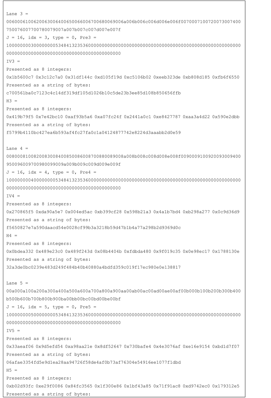
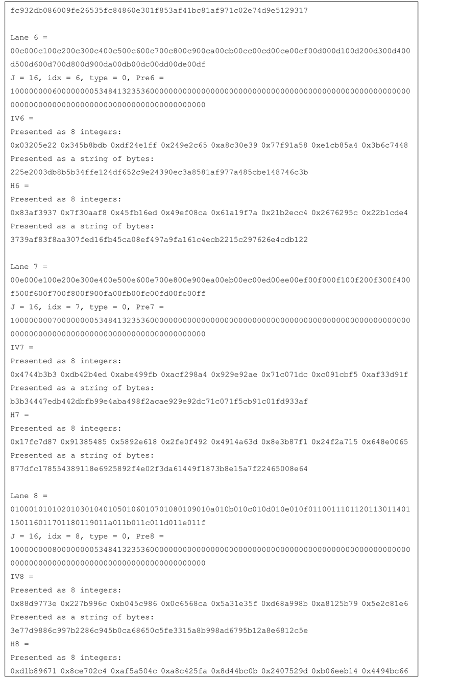
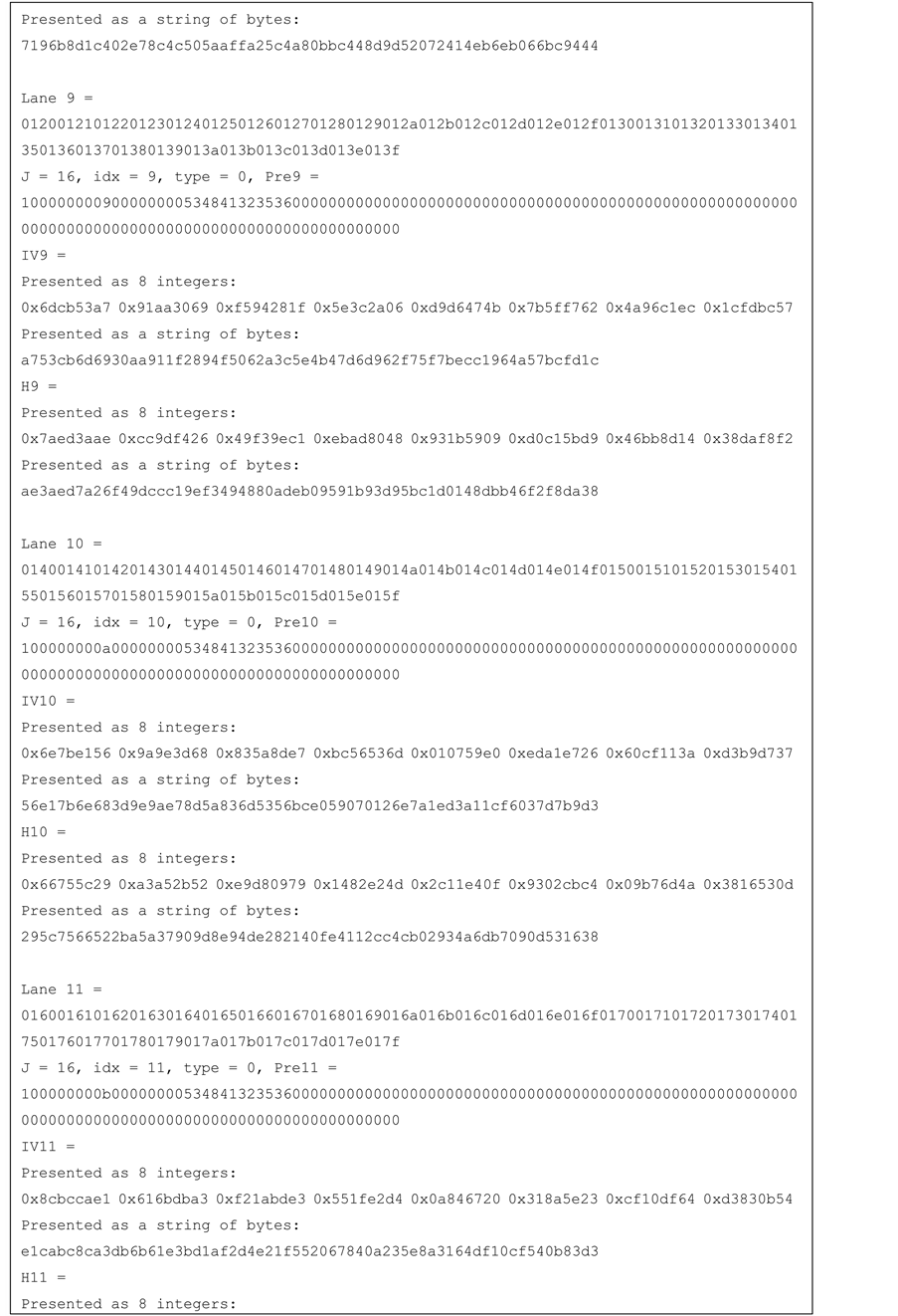
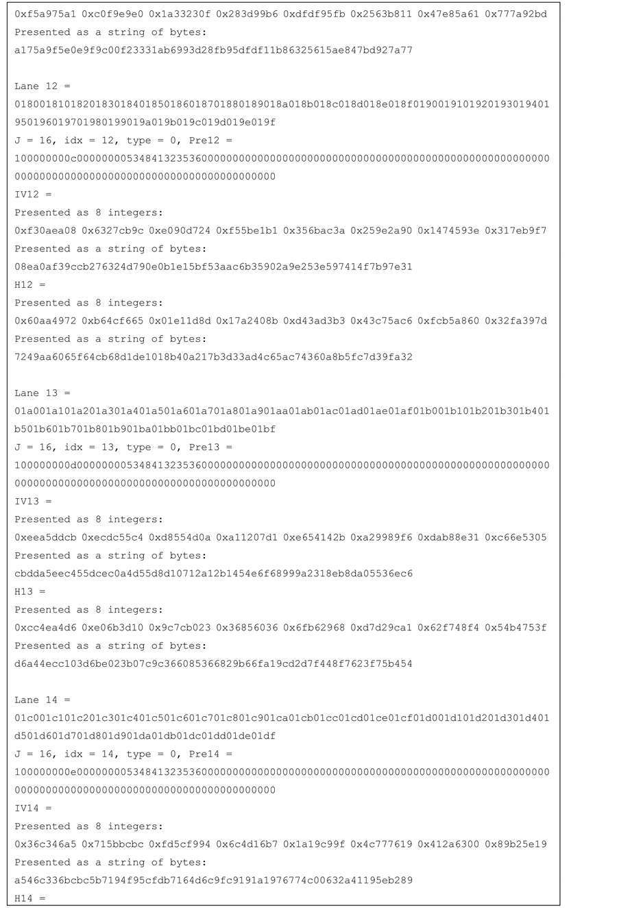
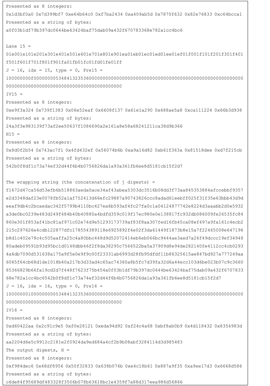
Figure 12. Test vector for SHA-256 16-lanes.