Journal of Modern Physics
Vol.08 No.06(2017), Article ID:76499,16 pages
10.4236/jmp.2017.86056
Fundamental Concept of Interdiffusion Problems
Takahisa Okino1*, Hiroki Cho2, Kazu-Masa Yamada3
1Applied Mathematics Department, Faculty of Engineering, Oita University, Oita, Japan
2Department of Mechanical Systems Engineering, Faculty of Environment Engineering, University of Kitakyushu, Kitakyushu, Japan
3Department of Production Systems Engineering, National Institute of Technology Hakodate College, Hakodate, Japan

Copyright © 2017 by authors and Scientific Research Publishing Inc.
This work is licensed under the Creative Commons Attribution International License (CC BY 4.0).
http://creativecommons.org/licenses/by/4.0/


Received: April 7, 2017; Accepted: May 21, 2017; Published: May 26, 2017
ABSTRACT
In accordance with the definition of diffusivity, the origin of coordinate system of the original diffusion equation is set at a point in the solvent material. Kirkendall revealed that Cu atoms, Zn atoms and vacancies move simultaneously in the interdiffusion region. This indicates that the original diffusion equation is a moving coordinate system for the experimentation system outside the diffusion region. The diffusion region space which means vacancies and interstices among atoms plays an important role in the diffusion phenomena. The theoretical equation of the Kirkendall effect is reasonably obtained as a shift between coordinate systems of the diffusion equation. The situation is similar to the well-known Doppler effect in the wave equation. Boltzmann transformed the original diffusion equation of a binary system into the nonlinear ordinary differential equation in accordance with the parabolic law. In the previous works, the solutions of the diffusion equation transformed by Boltzmann were analytically obtained and we found that the well-known Darken equation is mathematically wrong. In the present study, we found that the so-called intrinsic diffusivity corresponds in appearance to the physical solution obtained previously. However, the intrinsic diffusivity itself conceived in the diffusion research history is essentially nonexistent.
Keywords:
Interdiffusion, Intrinsic Diffusion, Kirkendall Effect, Parabolic Law

1. Introduction
The heat conduction equation proposed by Fourier in 1822 has been applied to investigating the temperature distribution in materials [1] . In 1855, Fick directly applied the heat conduction equation to diffusion phenomena [2] . As far as the shape of heat conduction material is unchangeable during a thermal treatment, the coordinate system of heat conduction equation set in a material is a fixed one, since the coordinate system is not influenced by the variation of internal structure in the material. Here, we should notice that the concentration of diffusion particles is a real quantity in physics, although the temperature is a thermodynamic state quantity. It is thus considered that the coordinate system of diffusion equation set in the diffusion field (solvent) is generally a moving one, since the origin of coordinate system is influenced by a variation of the diffusion field. It is thus indispensable for understanding the diffusion problems to discuss their coordinate systems, since the diffusion particles, solvent particles and also the diffusion region space which means vacancies and interstices among atoms move simultaneously against a fixed point outside the diffusion system.
When the Fick’s laws were proposed, the Gauss’s divergence theorem had been already reported in 1840 [3] . Nevertheless, the problem of coordinate system of diffusion equation was not mathematically investigated in accordance with the divergence theorem in those days. The problems of the coordinate transformation relevant to the diffusion equation had not been thus discussed in the diffusion history for a long time before the previous work [4] . The new findings, which are extremely dominant in the diffusion study, were reasonably obtained through the coordinate transformation theory then.
It seems that the new fundamental findings different from the existing diffusion theories may exert a great influence on the actual diffusion problems, just because of the fundamental findings themselves. For example, one of them reveals that the well-known intrinsic diffusion concept is unnecessary for understanding the interdiffusion phenomena [5] . However, those findings have not yet been universally known in the concerned research field [6] [7] [8] . That is the very reason to perform the present work in accordance with an entirely different viewpoint from the previous work.
The solutions of a typical interdiffusion problem were already obtained as analytical expressions in accordance with results of the well-known Boltzmann Matano method [9] [10] [11] . Using the analytical solutions for the interdiffusion problems, the fundamental problems of diffusivities and diffusion fluxes are discussed in accordance with the mathematical theory. In the present work, the original meaning of the so-called interdiffusion coefficient and that of the intrinsic diffusion coefficient misunderstood for a long time will be thus clarified in the following.
2. Raft Model of Interdiffusion Problems
In accordance with the definition of diffusivity, the origin of coordinate system of the original diffusion equation is set at a point in the solvent material. In 1947, Kirkendall revealed that Cu atoms, Zn atoms and vacancies move simultaneously in the interdiffusion region [12] . This indicates that the original diffusion equation is a moving coordinate system for the experimentation system outside the diffusion region. A discussion on the relation between the coordinate systems of diffusion equation is indispensable for understanding diffusion phenomena [4] . Analyzing interdiffusion problems is thus considerably complicated. In the following, as an example of problems between coordinate systems, we discuss motions of persons on a raft floating on a pond before the discussion about interdiffusion problems.
The water in a pond is at rest and a rectangle raft of mass , length
  and width
  floats also at rest in the pond. As shown in Figure 1, the diagonal lines intersect each other at the point
  then. The origin of
  axis along the length direction is set at the point
  on the raft. Persons A and B with mass
  and mass
  who are at rest on the line
  at the initial time
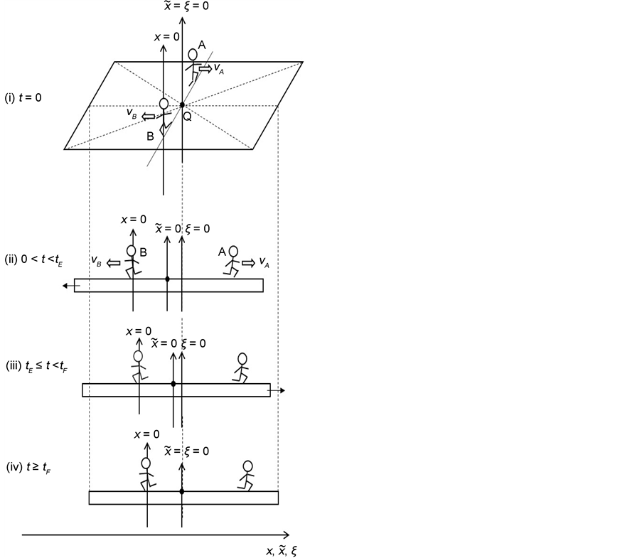
Figure 1. Raft model of interdiffusion phenomena. The persons A and B on the raft correspond to the mass center of diffusion particles and that of solvent ones. The raft and water in a pond correspond to the diffusion region space and the free space near the specimen surface of diffusion region. (i) The time  corresponds to the initial state of diffusion system. (ii) The time interval
  corresponds to a diffusing state at a high temperature. (iii) The time interval
  corresponds to a state of the diffusion system during temperature fall and it reaches a thermal equilibrium state at
  in the given room temperature. (iv) The time regions
  correspond to the final state after diffusion treatment.
start walking with an arbitrary velocity for  in the opposite direction from each other. Under the condition of
 , the origin of
  axis parallel to the
  axis is set at the point
  of the mass center of the persons. Under the condition of
 , the origin of
  axis parallel to the
  axis is set at a point
  on the bank beside pond on the line
  in the initial state.
In the following, we discuss the motion of person A in the isolated system composed of the raft and persons using each of the coordinate systems,  ,
,  and
and , under the initial condition
  at
at .
.
In an arbitrary time between , we conceive that the persons A and B move in the opposite direction from each other with arbitrary velocities
  and
and  against the point R and that they stop walking on the raft at the same time
 . In that case, the law of momentum conservation yields
 (1)
(1)
in the isolated system of the raft and persons, where  is a velocity of the raft against the point R. The mass center in the isolated system is immobile against the point R in accordance with the physical theory then, even if the raft moves against the point R. In other words, the raft moves in accordance with the motion of the persons like the concerned mass center is continually immobile against the point R.
The velocities of persons A and B,  and
and , against the point Q are obtained as
 (2)
(2)
The relative velocity  between persons A and B are then expressed as
 ,
,
and it does not depend on the coordinate systems  and
and .
.
The migration length of raft between  from the point R is expressed as
 .
.
When the persons on the raft stop walking at the same time , the relation of
  leads to that of
  then. If the velocity of water flow
  satisfies the relation given by

the raft returns to the initial position and it has been at rest ever since. The mass center of the isolated system is shifted from the initial state  to
to  then.
then.
In the present model, it is thus indispensable for understanding the motion of person A against the point R to investigate the behavior of the raft and water in the pond. In other words, it is apparent that we cannot understand the motion of person A against the point R only from the relative motion between the persons A and B on the raft.
3. Binary System Interdiffusion
As is known from the unified theory of diffusion problems, the basic concept of diffusion phenomena is in the interdiffusion problems [4] . In the following discussion, the above raft model is reasonably applied to a typical binary system interdiffusion problem in accordance with the mathematical physics. In that case, the person A, the person B, the raft and water in the pond correspond to the mass center of diffusion particles, the mass center of solvent particles (diffusion field), the diffusion region space, and space of the diffusion region outside, respectively. Here, note that the diffusion region space and the space of diffusion region outside have no mass, whereas the raft and water in the pond have the mass  and a mass.
Metal plates A and B with a uniform cross section  are composed of elements I and II for each other. The concentrations of I and II in the metal plate A are
  and
and  and their diffusivities are
  and
and  in the initial state, respectively. The concentrations and diffusivities in the metal plate B are similarly
 ,
,  ,
,  and
and . In general, those values of concentration and diffusivity are different from each other. In the following, we discuss the interdiffusion problem in the diffusion couple composed of the metal plates A and B.
As shown in Figure 2, the diffusion couple is smoothly jointed at the interface between A and B. The coordinate axis  perpendicular to the cross section
  is defined as
  direction. The origin of
  axis is set at the point
  of a mass center of diffusion field
  for
for  on the initial interface then. In the same manner, the origin of coordinate axis
  parallel to the
  axis is set at a point
  of space on the initial interface. Further, the origin of coordinate axis
  parallel to the
  axis is set at a point
  on the line
  outside the diffusion system in the initial state.
Since the diffusivity depends on an interaction between a diffusion particle and the diffusion field near the diffusion particle itself, the basic diffusion equation with the diffusivity is expressed by the time and space coordinate . In relation to the raft model, however, the diffusion equations expressed by the coordinates
  and
and  are necessary for understanding the diffusion phenomena, since the basic diffusion equation is relevant to the relative motion between collective particles of elements I and II. In the present case, the problems of the coordinate transformation of diffusion equation are thus discussed under the initial condition
  at
at .
.
We denote the concentrations and diffusivities of I and II by ,
,  ,
,  and
and  in the diffusion region
  during a thermal diffusion. In that case, their boundary values are physically accepted as constant values,
  ,
,  ,
,  and
and  at
at  and
and ,
,  ,
,  and
and  at
at , during a thermal diffusion. Those values are thus used as boundary values for the partial
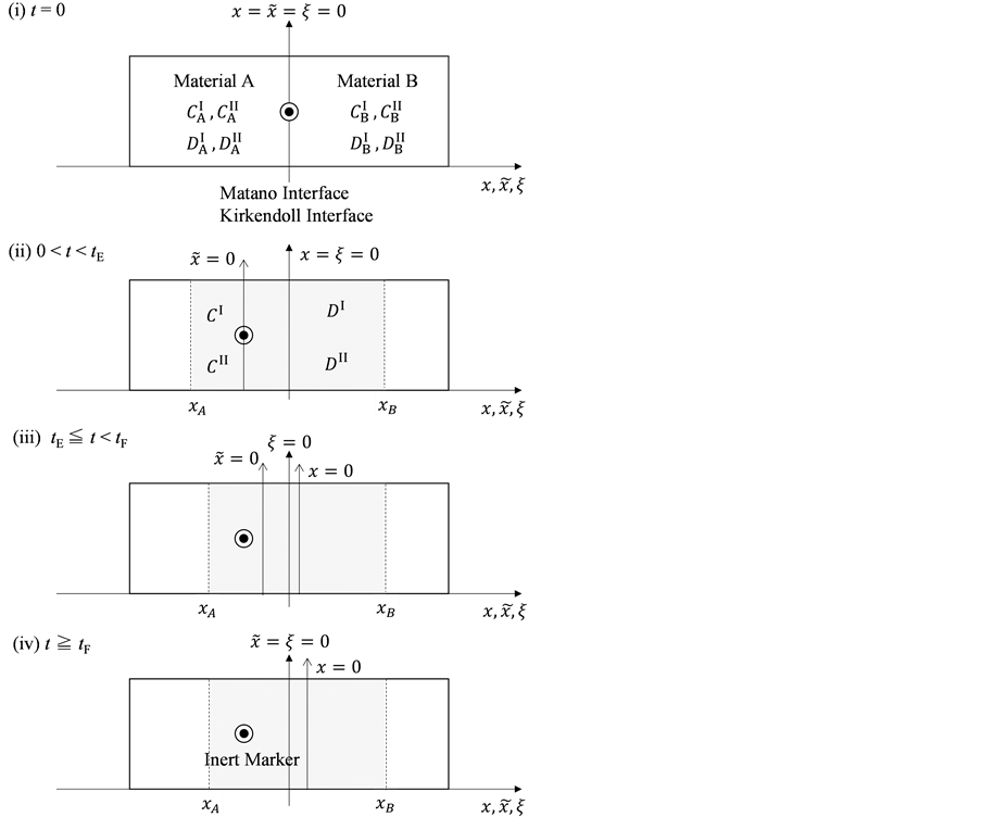
Figure 2. Typical interdiffusion problem of a diffusion couple. The metal plates A and B composed of elements I and II were used for a diffusion couple. Their diffusivities and concentrations are  and
and  in the initial state. Those values during thermal diffusion are
  in the diffusion region. The inert marker denoted in the figure moves during the diffusion process because of its inert characteristic. The time intervals of (i) - (iv) correspond to those of Figure 1, respectively.
differential equations of diffusion.
The basic diffusion equations of I and II are expressed as
 (3)
(3)
Since the shape variation of diffusion couple is negligible in the usual experimentation, the total particle numbers of I and II on an arbitrary cross section in the diffusion region are considered to be constant with a good approximation. In the typical interdiffusion problems, the relation of
 (4)
(4)
is thus generally accepted regardless of the coordinate systems, where the normalized concentrations are used.
Substituting (4) into (3) yields

and it is rewritten as
 (5)
(5)
In accordance with the theory of partial differential equation, (5) means that the relation of

must be valid using an arbitrary function  of t because of
 . In the present case, the differential equation is only for
  in accordance with the mathematical theory. In other words, the relation of
  is thus valid because of
  in the diffusion region.
Their diffusivities are thus commonly expressed as
 (6)
(6)
only in the partial differential equation (3). However, note that it is not generally valid in the actual diffusion phenomena when we substitute the initial and/or boundary values,  ,
,  ,
,  and
and , into their general solutions
  and
and  of (3). Substituting (6) into (3) yields
 (7)
(7)
where the suffix  is removed because the general solutions are mathematically in common. Here,
  at
at  and
and  at
at  are formally used in common for the elements I and II as initial and boundary values of the general solutions of (7).
The Gauss’s divergence theory shows that the diffusion flux of basic diffusion equation (7) is obtained as
 (8)
(8)
by integrating it with respect to  because of
 . Here,
  is the well-known Fickian first law and
  independent of the time and space is the intrinsic diffusion flux defined by the previous work [13] . The intrinsic diffusion flux
  plays an important role in the self-diffusion theory of
  and it has a relation with a self-diffusion coefficient
  yielding
 ,
,
where  and
and  are a concentration and a lattice constant in a pure material [4] .
Substituting (4) into the Fickian first law , the relation of
 (9)
(9)
is valid only in the partial differential equation (3). Further, it is clarified that the relation of
 (10)
(10)
is valid in the self-diffusion theory in [4] . Equations (8), (9) and (10) yield
 (11)
(11)
which is valid only in the partial differential equation (3).
When the origin  of
of  axis moves with the velocity
  against the origin
  of
of  axis, (7) is transformed into the equation of
 (12)
(12)
in the fixed coordinate system outside the diffusion system. Here, the relations of differential operators yielding

are used for (7), where the relations of
 and
and 
are valid between the coordinate systems  and
and .
.
4. Solutions of Nonlinear Diffusion Equation
It is generally considered that the diffusivity  of the element I or II between
  depends on the coordinate system
  because of the concentration dependence. In that case, we cannot analytically solve the nonlinear partial differential equation (7) as it is.
In 1894, Boltzmann transformed (7) into the nonlinear ordinary differential equation of
 (13)
(13)
using the relation  of the parabolic law [9] . Further, (13) can be rewritten as
 (14)
(14)
where the relation of

is used [11] [14] . Equation (14) is considered to be a diffusion flux in the parabolic space. In mathematics, that the diffusivity depends on the coordinate system yields the relation of
 (15)
(15)
The general solutions of (13) were obtained as analytical expressions yielding
 (16)
(16)
 (17)
(17)
where (14) and (15) were simultaneously calculated using the integral constants ,
,  ,
,  and
and  in common for the elements I and II [11] . The notation of
  is used as
  for
for  and
and  for
for . The other notations used here for the general solutions are as follows:

When we substitute the boundary values,  ,
,  ,
,  and
and , for
, for  in the concerned diffusion system into the general solution of (16) and (17), the physical solutions of (3), i.e.,
  and
and  are obtained as
 (18)
(18)
 (19)
(19)
between , because of
 . The notations used here are as follows:


Substituting the initial and/or boundary values into the general solutions of the diffusion equation (13) i.e., (16) and (17), the physical solutions of the diffusion equation (3) were reasonably obtained as (18) and (19). As can be seen from figure 3 and figure 4 in [11] , the present solutions agree with the results of the Boltzmann Matano method. Further, it is clarified that the physical solutions of (18) and (19) are equivalent to those of (12) because of  in the actual interdiffusion problems as discussed later. In order to understand the interdiffusion phenomena, however, we must further investigate the behavior of the diffusion region space corresponding to the movement of the raft as mentioned above, since the diffusion flux of (3) is different from that of (12) as discussed in detail later even if
  is valid.
The diffusivities  and
and  in the diffusion region shown in Figure 2 are generally different from each other because of the concentration dependence of diffusivity caused by a difference between
  and
and . The physical solution of (18) obtained here shows that the relation of
 (20)
(20)
is valid between . At the same time, the relation of
 (21)
(21)
is generally valid between the diffusion fluxes obtained by using (18) and (19).
Here, note that the difference between (6) and (20) or (9) and (21) has been ignored in the diffusion history. We believe that the Kirkendall effect (K effect) is caused by the relation of (21) [12] . At the same time, as discussed later, we cannot accept the concept of intrinsic diffusion developed in the diffusion history.
In a word, the usual diffusivities  and
and  shown in Figure 2 have been thus named as an interdiffusion coefficient
 , where (6) is valid only in a partial differential equation of diffusion, and the concept is acceptable then. On the other hand, diffusivities
  and
and  obtained as physical solutions of (18) correspond in appearance to ones named as intrinsic diffusion coefficients from a different viewpoint in those days. Based on the above theory, however, the concept of intrinsic diffusion coefficients is not acceptable, since it is apparent that there is no such especial diffusivity in the concerned diffusion region.
The so-called Darken equation relevant to the interdiffusion coefficient and the intrinsic diffusion coefficients has been used for analyzing interdiffusion problems for a long time [15] . However, we cannot mathematically accept the relation among the interdiffusion coefficient  and the intrinsic diffusion coefficients
  and
and  in accordance with the above discussion. Here, we should notice that the Darken equation is also mathematically wrong in the derivation process [5] .
5. Flux of Diffusion Region Space
The concept of diffusion flux is useful for understanding of diffusion phenomena. The diffusion flux of the diffusion region space plays an important role to understand interdiffusion phenomena like the motion of persons in the raft model depends on the motion of raft.
The Gauss’s divergence theory shows that the diffusion flux is obtained as
 (22)
(22)
by integrating the diffusion equation (12) with respect to . Here,
  is an integral constant because of
 .
.  is a diffusion flux of the diffusion region space caused by the migration of diffusion particles and/or solvent ones and it can be observed only from using the coordinate system
  outside the diffusion system.
Using the velocity  of the origin
  of
of  axis against the origin
  of
of  axis, the diffusion equation is obtained as
 (23)
(23)
and the diffusion flux is
 (24)
(24)
Here, note that the diffusion fluxes of (8), (22) and (24) are valid only in the partial differential equations (7), (12) and (23), respectively. When (8), (22) and (24) are applied to the elements I and II, the relation among diffusion fluxes of
 (25)
(25)
is physically valid as a relation between the inside flux of the diffusion region and the outside one, where ,
,  and
and .
.
Equation (25) yields the relation of
 (26)
(26)
since ,
,  and (4) are valid regardless of the coordinate systems. The diffusion flux of
  means the flux of diffusion particles and solvent ones caused by the coordinate transformation, where
  is the velocity of the origin
  of
of  axis against the origin
  of
of  axis. The relation of
 (27)
(27)
is thus valid, since the diffusion region space moves in the opposite direction against the diffusion particles.
Equations (26) and (27) yield a physically reasonable relation of
 (28)
(28)
to be valid among the velocities of the coordinate systems.
6. Kirkendall Effect
In general, the diffusion experiments are performed at a high temperature between  shown in Figure 2 and the temperature of experimental specimen becomes gradually a room temperature between
 . The diffusion region space interacts with the free space outside the diffusion system then and subsequently the diffusion system becomes a thermal equilibrium state at
 , where the entropy maximization principle and the free energy minimum principle stand against each other between
 . As can be easily seen, the situation corresponds to the motion of the raft and water flow between
  in Figure 1.
The interface  is the so called Matano interface (M interface) whereas the interface
  is called the Kirkendall interface (K interface) in the metallurgy field. The number of diffusion particles through the M interface is equal to that of solvent particles, since the shape variation of diffusion system is not observed in usual experiments. It seems that the M interface is immobile after a thermal diffusion process in accordance with many experimental results.
It is considered that the diffusion region is an isolated system and the mass center is immobile between . In other words, the M interface is the mass center of diffusion region in the initial state and the diffusion region space moves like the M interface is immovable between
  in a similar way to the mass center in the raft model in Figure 1. Subsequently, the diffusion region space moves with the temperature fall in a similar way to the movement of raft between
 . In that case, the diffusion system gradually reaches a thermal equilibrium state at a room temperature. However, the mass center is still immovable between
 , since the diffusion region space has no mass.
The coordinate origin set at a point P on the M interface in the initial state is also immovable, since the M interface is immovable. In other words, the relation of  is reasonably valid in the present diffusion system. In that case, (28) yields
 (29)
(29)
because of .
.
Here, using the initial and/or boundary values for (24), the relation yielding
 (30)
(30)
is reasonably obtained (See Appendix).
An inert marker set at the K interface moves in accordance with the flow of diffusion region space between  because of the characteristic of the inert marker itself. The K interface returns subsequently to the initial position of
  between
 , since the diffusion region space interacts with the free space outside the diffusion system like the diffusion system becomes a thermal equilibrium state. It is considered that the diffusion region space interacts with the free space near the specimen surface between
 . Thus, the marker does not move in the
  axis direction then, since the diffusion region space moves in the surface direction perpendicular to the
  axis. The migration length of diffusion region space in the
  axis direction is thus still visualized by the marker position.
Based on the above mentioned, the migration length of an inert marker is expressed as
 (31)
(31)
at  in accordance with the shift between the coordinate systems
  and
and . The diffusion equation (7) is equal to (12) because of
 , although the diffusion flux of (8) is different from that of (22) even if
 . In that case, therefore, the inert marker exists at a point of
  in the coordinate system of the diffusion region outside. This is the so-called K effect
 . Here, it is revealed that the K effect is caused by the shift between the coordinate systems
  and
and  in a similar way to the well-known Doppler effect in the wave equation.
For an arbitrary time , the empirical relation of K effect given by
 (32)
(32)
is well known, where  is a constant determined from the concerned experimental results. The above theoretical equation of K effect is then written as
 (33)
(33)
Equation (33) shows that the K effect depends not only on the initial diffusivity values but also on the initial concentration values. Here, (33) is derived by using  in Appendix. Therefore, we need reexamine a
  value by using the relation of
 (34)
(34)
so as to agree with the empirical equation (32).
Hereinbefore, the Kirkendall effect was reasonably explained by the present interdiffusion theory, regardless of the intrinsic diffusion concept. It was thus revealed that the diffusion region space plays an important role in the interdiffusion problems. At the same time, the discussions of setting coordinate system of diffusion equation are essentially dispensable for understanding the diffusion phenomena.
7. Discussion
The diffusion study is an important subject relevant to basic problems in the fabrication process of materials such as alloys, semiconductors, functional materials, and so on. Their diffusion problems in detail have been thus widely investigated in accordance with the industrial requirement for a long time. However, some unsolved problems relevant to the fundamental nonlinear diffusion equation, which are extremely dominant in mathematical physics, have been still leaved in the diffusion history. In the cause of them, the physical interpretation of the K effect has been misunderstood for a long time.
As is well known, the physical solutions of a partial differential equation are determined from substituting the given initial and boundary values into the general solutions in mathematics. The difference between the physical solutions and the general solutions in mathematics has been confused in the diffusion history. For example, the expression of the diffusion flux  using the general solutions is thus apparently different from
  using the physical solutions. Using the expression of the interdiffusion coefficient
  of the general solutions and the diffusivity
  for
for  of the physical solutions, the well-known Darken equation is expressed as
 (35)
(35)
Based on the present mathematical theory, (35) is apparently wrong, since the left-hand side is a general solution whereas the right-hand is expressed by using physical solutions. Further, it is also revealed that the Darken equation is mathematically wrong in the derivation process [5] .
8. Conclusions
It had been considered for a long time that the analytical solutions of (3) are impossible. However, we could reasonably obtain the general solutions of (13) as (16) and (17). In other words, the physical solutions of (3) were analytically obtained as (18) and (19). In the present work, the fundamental concept of interdiffusion phenomena was reasonably clarified in accordance with the mathematical theory. Further, the analytical method discussed in the present work is reasonably applicable to an interdiffusion problem of many elements system [16] .
Here, the present results yield the following conclusions.
1) In general, the discussion about setting the coordinate systems of diffusion equation in the diffusion problems is essentially necessary for understanding of the diffusion phenomena.
2) An element in the interdiffusion region has only one diffusivity value. The so-called interdiffusion coefficient means the unsolved one in the partial differential equation. On the other hand, the intrinsic diffusion coefficient corresponds to the solved one using the given initial and boundary values for the general solutions. Therefore, such an especial intrinsic diffusion coefficient conceived in the diffusion history is essentially nonexistent in accordance with the mathematical theory.
In view of the influence of misunderstanding problems pointed out here on the younger, we hope that the conclusions are universally known in the concerned research field as soon as possible, just because of the fundamental matters themselves.
Cite this paper
Okino, T., Cho, H. and Yamada, K.-M. (2017) Fundamental Concept of Interdiffusion Problems. Journal of Modern Physics, 8, 903-918. https://doi.org/10.4236/jmp.2017.86056
References
- 1. Fourier, J.B.J. (1822) Analytique de la Chaleur. Didot, Paris, 499-508.
- 2. Fick, A. (1855) Philosophical Magazine, 10, 31-39.
- 3. Gauss, C.F. (1840) Resultateaus den Beobachtungen des Magnetishen Vereins, 4, 1.
- 4. Okino, T. (2015) Journal of Modern Physics, 6, 2109-2144.
https://doi.org/10.4236/jmp.2015.614217 - 5. Okino, T. (2013) Journal of Modern Physics, 4, 1495-1498.
https://doi.org/10.4236/jmp.2013.411180 - 6. Haug, K., Keiser, D. and Sohn, Y. (2013) Metallurgical and Materials Transactions A, 44, 738-746.
https://doi.org/10.1007/s11661-012-1425-9 - 7. Kuhn, P., Horbach, J., Kargl, F. and Meyer, A.Th. (2014) Physical Review B, 90, Article ID: 023409.
https://doi.org/10.1103/PhysRevA.90.023409 - 8. Paul, T.R., Belova, I.V., Levchenko, E.V., Evteev, A.V. and Murch, G.E. (2015) Diffusion Foundations, 4, 25-54.
https://doi.org/10.4028/www.scientific.net/DF.4.25 - 9. Boltzmann, L. (1894) Annual Review of Physical Chemistry, 53, 959-964.
https://doi.org/10.1002/andp.18942891315 - 10. Matano, C. (1933) Japanese Journal of Applied Physics, 8, 109-113.
- 11. Okino, T. (2011) Materials Transactions, 52, 2220-2227.
https://doi.org/10.2320/matertrans.M2011137 - 12. Smigelskas, A.D. and Kirkendall, E.O. (1947) Transactions of the Metallurgical Society of AIME, 171, 130-142.
- 13. Okino, T. (2012) Journal of Modern Physics, 3, 1388-1393.
https://doi.org/10.4236/jmp.2012.310175 - 14. Okino, T. (2012) Journal of Modern Physics, 3, 255-259.
https://doi.org/10.4236/jmp.2012.33034 - 15. Darken, L.S. (1948) Transactions of the Metallurgical Society of AIME, 175, 184-201.
- 16. Okino, T. (2014) Applied Physics Research, 6, 1-7.
https://doi.org/10.5539/apr.v6n2p1
Appendix
Even if the diffusion couple satisfies  in the diffusion system shown in Figure 2, the generality of diffusion system holds still. In that case, the particles of element I diffuse from the interface at
  into the diffusion region between
 . On the other hand, the particles of element II diffuse from the interface at
  into the diffusion region between
 . The diffusion junction depths
  and
and  are estimated as
 and
and , (A-1)
where  is a parameter and
  is tentatively adopted in the present work.
Using (A-1) and the concentration difference of boundary values
 and
and , the actual diffusion fluxes of elements I and II are expressed as
 (A-2)
(A-2)
Equation (A-2) yields
 (A-3)
(A-3)
The diffusion flux of (A-3) caused by the coordinate transformation corresponds to the flux of diffusion region space given by
 (A-4)
(A-4)
since the flux of diffusion region space moves in the opposite direction to the diffusion flux of (A-3). Substituting (A-4) into (29) yields
 (30)
(30)

Submit or recommend next manuscript to SCIRP and we will provide best service for you:
Accepting pre-submission inquiries through Email, Facebook, LinkedIn, Twitter, etc.
A wide selection of journals (inclusive of 9 subjects, more than 200 journals)
Providing 24-hour high-quality service
User-friendly online submission system
Fair and swift peer-review system
Efficient typesetting and proofreading procedure
Display of the result of downloads and visits, as well as the number of cited articles
Maximum dissemination of your research work
Submit your manuscript at: http://papersubmission.scirp.org/
Or contact jmp@scirp.org