Journal of Modern Physics
Vol.3 No.4(2012), Article ID:18899,12 pages DOI:10.4236/jmp.2012.34044
An Introductory Study of the Hydrogen Atom with Paraquantum Logic
1Group of Applied Paraconsistent Logic, Santa Cecília University, Santos, Brazil
2Institute for Advanced Studies, University of São Paulo Cidade Universitária, São Paulo, Brazil
Email: inacio@unisanta.br
Received January 3, 2012; revised February 28, 2012; accepted March 12, 2012
Keywords: Paraconsistent Logic; Paraquantum Logic; Classical Physic; Relativity Theory; Quantum Mechanics
ABSTRACT
Paraquantum Logics (PQL) has its origins in the fundamental concepts of the Paraconsistent Annotated Logics (PAL) whose main feature is to be capable of treating contradictory information. Based on a class of logics called Paraconsistent Logics with annotations of two values (PAL2v), PQL performs a logical treatment on signals obtained by measurements on physical quantities which are considered Observable Variables in the physical world. In the process of application of the PQL the obtained values are transformed in Evidence Degrees and represented on a Lattice of four Vertices where special equations transform these degrees into Paraquantum logical states ψ which propagate. The propagation of Paraquantum logical states provides us with results which can be interpreted and modeled through phenomena studied in physics. Using the Paraquantum equations, we investigate the effects of balancing of Energies and the quantization and transience properties of the Paraquantum Logical Model in real Physical Systems. As a demonstration of the usage of the Paraquantum equations we perform a numerical comparative study that applies the PQL to the Bohr’s model to find the energy levels of the Hydrogen atom. It is verified that the values of energy in each level of the Paraquantum logical model of the Hydrogen atom are close to the values found by the conventional way. The results through the Paraquantum Logic allow considering other important properties of the atom, as the forecast of number of electrons in each layer.
1. Introduction
The conception of physical system models that prove to be more efficient in order to respond to the analyses in extreme conditions becomes necessary when we verify inconsistencies in computation obtained from models which reproduce the same natural phenomenon but are from different areas of physics (see [1,2]). In order to create a mathematical tool that conveniently make these results compatible, we present in this paper a model based on the concepts of a non-Classical logics called Paraconsistent Logics (PL) (see [3,4]).
A Paraconsistent Logic is a non-classical logic which revokes the principle of non-Contradiction and admits the treatment of contradictory information in its theoretical structure (see [4,5]). The foundational principles of the Paraconsistent Logics can be seen with details in [1] and [4]. In [5] we presented an interpretation of the Paraconsistent Logic that it resulted in the foundations of an applicable model in physical systems. This extension of the PL was denominated of Paraconsistent Annotated Logic with annotation of two values (PAL2v). The PAL2v is a class of Paraconsistent Logics particularly represented through a Lattice of four vertices and from its foundations the Paraquantum Logics (PQL) was created.
The organization of the paper is as follows: in the Section 2 the basic concepts, the interpretation and the main equations of the LPA2v Logic are presented. In Section 3 the main concepts of the Paraquantum Logic are presented. In the Section 4 a Paraquantum Logical Model is proposed to quantization of values of Physical Quantities. In Section 5 the Paraquantum Logical Model is applied for calculations of the Energy levels in the Hydrogen Atom. In the Section 6 are presented conclusions about the Paraquantum Logic application results in the Hydrogen Atom.
2. The Main Concepts of the Paraconsistent Annotated Logic with Annotation of Two Values (PAL2v)
According to [5] we can obtain through the PAL2v a representation of how the annotations or evidences express the knowledge about a certain proposition P. This is done through a lattice on the real plane with pairs (m, λ)which are the annotations. In this representation an operator is fixed: ~:|t| ® |t|
where t = {(m, λ) | m , λ Î [0, 1] Ì Â}.
If P is a basic formula then:
~ [(m, λ)] = (λ, m) where m, λ Î [0, 1] Ì Â.
The operator ~ stands for the “meaning” of the logical symbol of negation of the system to be considered.
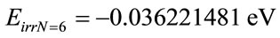
In applications for analyses of physical systems m is the Favorable Evidence Degree related to the Proposition P and λ is the Unfavorable Evidence Degree related to the Proposition P. See Figure 1.
A Paraconsistent logical signal of the information about measurements of real Physical Systems can be written as: P(μ, λ)
where: P is the proposition to be analyzed.
(m, λ) is the annotation composed by the two evidence degrees.
In an intuitive way we can affirm that:
PT = P(1, 1) → The annotation (m, l) = (1, 1) assigns intuitive reading that P is inconsistent.
Pt = P(1, 0) → The annotation (m, l) = (1, 0) assigns intuitive reading that P is true.
PF = P(0, 1) → The annotation (m, l) = (0, 1) assigns intuitive reading that P is false.
P^ = P(0, 0) → The annotation (m, l) = (0, 0) assigns intuitive reading that P is Indeterminate.
When the Paraconsistent universe is modeled in a Lattice of four vertexes the values of the evidence degrees obtained by measurements in the physical world will result in Paraconsistent logical states eτ.
In the internal point of the lattice which is equidistant from all four vertices, we have the following interpretation: PI = P(0.5, 0.5) → The annotation (m, l) = (0.5, 0.5) assigns intuitive reading that P is undefined.
The Equations of PAL2v
According to [5], with the values of x and y that vary between 0 and 1 and being considered in an Unitary Square on the Cartesian Plane (USCP), we can get linear transformations for a Lattice k of analogous values to the associated Lattice τ of the PAL2v. The following final transformation is obtained:
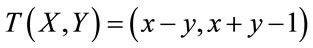 (1)
(1)
With the transformation (1) we can convert points of the USCP which represent annotations of τ into points of k which also represent annotations of τ (see [3-5]). According to the language of the PAL2v we have:
x = m → is the Favorable evidence Degree;
y = λ → is the Unfavorable evidence Degree.
The first coordinate of the transformation (1) is called Certainty Degree DC. So, the Certainty Degree is obtained by:
 (2)
(2)
The second coordinate of the transformation (1) is called Contradiction Degree Dct. So, the Contradiction Degree is obtained by:
 (3)
(3)
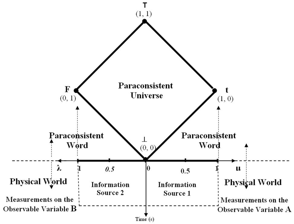
Figure 1. Representation of the paraconsistent universe in to lattice of four vertexes.
The second coordinate is a real number in the closed interval [–1, +1]. The y-axis is called “axis of the contradiction degrees”.
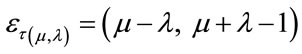
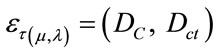
Since the linear transformation T(X, Y) shown in (1) is expressed with evidence Degrees μ and λ, from (2), (3) and (1) we can represent a Paraconsistent logical state eτ into Lattice τ of the PAL2v [4,5], such that:
 (4)
(4)
or
 (5)
(5)
where: eτ is the Paraconsistent logical state.
DC is the Certainty Degree obtained from the evidence Degrees μ and λ.
Dct is the Contradiction Degree obtained from the evidence Degrees μ and λ.
The Paraconsistent logical state eτ can be anywhere in the lattice τ, and a real Certainty Degree DCR can be obtained as follows:
For  we compute:
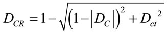 (6)
(6)
For  we compute:
 (7)
(7)
where:  and
and .
.
For DC = 0 we consider the undefined Paraconsistent logical state with: DCR = 0.
The resulting evidence degree which expresses the intensity of the Paraconsistent logical state ετ is computed by:
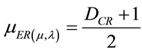 (8)
(8)
where:  is the resulting evidence Degree in function of μ and λ.
DCR is the real Certainty Degree calculated by (6) or (7).
3. The Paraquantum Logic (PQL)
In recent applications of the PAL2v equations there were the need of including restrictions in its algorithms (see [6,7]). The restrictions were necessary because under certain conditions the results obtained from the model changed through leaps or unexpected variations [7,8]. Later, it was seen in research based on PAL2v models that the application of its foundations offered results strongly connected to the ones found in modeling of phenomena studied in quantum mechanics (see [9,10]). With the same considerations used in the Paraconsistent logic (PAL2v) we can to define in the Lattice a Paraquantum logical state ψ.
A Paraquantum logical state ψ is created on the lattice of the PQL as the tuple formed by the certainty degree DC and the contradiction degree Dct [4]. Both values depend on the measurements performed on the Observable Variables in the physical environment which are represented by μ and λ [11,12]. Initially, we can express (2) and (3) in terms of μ and λ obtaining:
 (9)
(9)
 (10)
(10)
A Paraquantum function y(Py) is defined as the Paraquantum logical state y:
 (11)
(11)
For each measurement performed in the physical world of μ and λ, we obtain a unique duple  which represents a unique Paraquantum logical state ψ which is a point of the lattice of the PQL [11].
On the vertical axis of contradictory degrees, the two extreme real Paraquantum logical states are:
1) The contradictory extreme Paraquantum logical state which represents Inconsistency T:
 .
.
2) The contradictory extreme Paraquantum logical state which represents Undetermination ^:
 .
.
On the horizontal axis of certainty degrees, the two extreme real Paraquantum logical states are:
3) The real extreme Paraquantum logical state which represents Veracity t:
 .
.
4) The real extreme Paraquantum logical state which represents Falsity F:
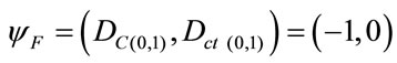 .
.
Inside of the Lattice each Paraquantum logical state, generated by , is related to a vector of state with the following characteristics:
The Vector of State P(ψ) will have origin in one of the two vertexes that compose the horizontal axis of the certainty degrees and its extremity will be in the point formed for the pair indicated by the Paraquantum function: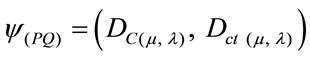 .
.
If the Certainty Degree is negative (DC < 0), then the Vector of State P(ψ) will be on the lattice vertex which is the extreme Paraquantum logical state False: ψF = (–1, 0).
If the Certainty Degree is positive (DC > 0), then the Vector of State P(ψ) will be on the lattice vertex which is the extreme Paraquantum logical state True: ψt = (1, 0).
If the certainty degree is nil (DC = 0), then there is an undefined Paraquantum logical state ψI = (0.0, 0.0).
The Vector of State P(ψ) will always be the vector addition of its two component vectors:
 Vector with same direction as the axis of the certainty degrees (horizontal) whose module is the complement of the intensity of the certainty degree:
 Vector with same direction as the axis of the contradiction degrees (vertical) whose module is the contradiction degree:
Given a current Paraquantum logical state ψcur defined by the duple  then we compute the module of a Vector of State P(ψ) as follows:
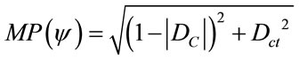 (12)
(12)
where: DC = Certainty Degree computed by (9), Dct = Contradiction Degree computed by (10).
Using (12) which is for computing the module of a Vector of State P(ψ), we have:
1) For DC > 0 the real Certainty Degree is computed by:
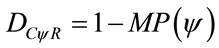 (13)
(13)
Therefore:
 (14)
(14)
where: DCψR = real Certainty Degree.
2) For DC < 0, the real Certainty Degree is computed by:
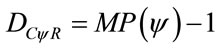 (15)
(15)
Therefore:
 (16)
(16)
where: DCψR = real Certainty Degree; DC = Certainty Degree computed by (9); Dct = Contradiction Degree computed by (10).
3) For DC = 0, then the real Certainty Degree is nil: .
.
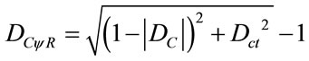
The intensity of the real Paraquantum logical state is computed by:
 (17)
(17)
The inclination angle ay of the Vector of State which is the angle formed by the Vector of State P(y) and the x-axis of the certainty degrees is computed by:
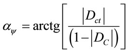 (18)
(18)
The degree of intensity of the contradictory Paraquantum logical state ψctrψ is computed by:
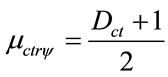 (19)
(19)
where: μctrψ = intensity degree of the contradictory Paraquantum logical state; Dct = Contradiction Degree computed by (10).
3.1. The Propagation of the Paraquantum Logical State ψ
There may be variations in the measurements performed on the observable variables in the physical environment which can dynamically change the values of the evidence degrees in such a way that the module of the Vector of State MP(ψ) tends to increase [11,12].
The propagation of the superposed Paraquantum logical states ysup through the lattice of the PQL happens due to the continuous measurements performed on the observable variables in the physical world. Since the Paraquantum analysis deals with favorable and unfavorable evidence degrees m and l of the measurements performed on the physical world, these variations affect the behavior and propagation of the superposed Paraquantum logical states ysup on the lattice of the PQL. When the module of the Vector of State MP(ψ) = 1, this vector will represent the maximal fundamental superposed Paraquantum logical states ψsupfmax which has real certainty degrees zero. The maximum Contradiction Degree for this condition is when the Vector of State P(ψ) forms an angle of 45˚ with the horizontal axis of certainty degrees. Therefore, given that the inclination angle of the Vector of State is α = 45˚ then the maximum Contradiction Degree for this condition is computed by:
 .
.
When the Vector of State has inclination angle α = –45˚, or still, with origin in the extreme Vertex representative of the extreme False Paraquantum logical state this same condition is found. In that extreme contradictory situation the module of the Vector of State MP(ψ) will have his maximum value of: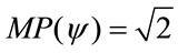 . The unbalanced contradictory Paraquantum logical state ψctru is the one located on the lattice of states of the PQL where there is a condition of opposite signs between the Certainty Degree (DC) and the real Certainty Degree (DCψR).
The Paraquantum logical states into limits of the Region of Uncertainty are identified with Factors of maximum limitation of transition [11]. These factors are:
1) The factor of Paraquantum limitation False/inconsistent—hQyFT.
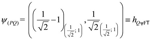
2) The factor of Paraquantum limitation True/inconsistent—hQytT.

3) The factor of Paraquantum limitation False/undetermined—hQyF^.
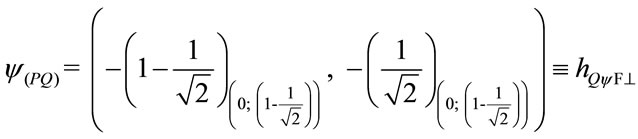
4) The factor of Paraquantum limitation True/undetermined—hQyt^.
All the Superposed Paraquantum logical states ysup to these and that they will have variation of the inclination angle until null degree delimit the Region of Uncertainty of the Lattice of PQL.
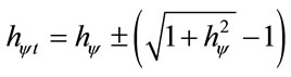
3.2. The Paraquantum Factor of Quantization hψ
When the superposed Paraquantum logical state ysup propagates on the lattice of the PQL a value of quantizetion for each equilibrium point is established. This point is the value of the contradiction degree of the Paraquantum logical state of quantization yhy [11] such that:
 (20)
(20)
where: hy is the Paraquantum Factor of quantization.
The factor hy quantifies the levels of energy through the equilibrium points where the Paraquantum logical state of quantization yhy, defined by the limits of propagation throughout the uncertainty of the PQL, is located. In a process of propagation of Paraquantum logical state y, we have that in the instant that the superposed Paraquantum logical state ysup reaches the representative points of the limiting factors of the uncertainty region of the PQL, the Certainty Degree (DC) remains zero but the real Certainty Degree (DCyR) will be increased or decreased from zero and this difference corresponds to the effect called of the Paraquantum Leap [11,12]. So, on the point where the logical state of Paraquantum quantization yhy is located, we observe that in the instant of the arrival of the superposed logical states, the Certainty Degree (DC) will be zero but the real Certainty Degree (DCyR) will be increased corresponding to the Paraquantum Leap. In the same way, in the beginning of the propagation, therefore, at the instant that the superposed Paraquantum logical state ysup leaves the point where the logical state of Paraquantum quantization yhy is located, the Certainty Degree (DC) will be zero but the real Certainty Degree (DCyR) will be decreased according to the Paraquantum Leap. We observe that with respect to the point of Indefinition which is equidistant from the vertices of the PQL, therefore around the Paraquantum logical state of pure Indefinition yIP, the variation of values inside the limits can be expressed by [11,12]:
 (21)
(21)
These logical states establish connection in the point where the logical Paraquantum state of quantization yhy is situated. At the instant that the superposed Paraquantum logical states ysup visit the Paraquantum logical state of quantization yhy, the real Certainty Degree will have variations of the form:
 (22)
(22)
When the Paraquantum logical states ysup visit the Paraquantum state of quantization yhy established by the Paraquantum Factor of quantization hy, the Paraquantum Leap happens. The Equation (21) that relates the Paraquantum Logical states indicates that the Uncertainty Region of PQL is dependent of the level of transition frequency N that acts in the Paraquantum Factor of Quantization hψ, such that:
 (23)
(23)
N = integer positive ≥ 1 where: ΔψIP = variation around the Paraquantum logical state of Indefinition pure.
N = level of contraction frequency, or number of times of application of hψ.
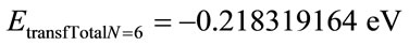
Figure 2 shows the interconnections between the factors and its characteristics, in which they delimit the Region of Uncertainty in the Lattice of PQL and the Paraquantum Leap in the propagation of the Paraquantum logical state y.
3.3. Action of the Paraquantum Factor of Quantization in the Fundamental Lattice of the PQL
The contraction of the Fundamental Lattice points out that the a Paraquantum Logical state ψ is an infinitely contracted Fundamental Lattice and has, through the Paraquantum Factor of Quantization hψ, all features of the PQL Fundamental Lattice. Since the propagation of the Superposed Paraquantum Logical states always occurs through the Paraquantum Logical state of Quantization ψhψ, given any point of the PQL Fundamental Lattice, this point will be the Paraquantum Logical state of Quantization ψhψ of the contracted Local Lattice. In order to completely express it, we have to take into account the factor related to the Paraquantum Leaps which will be added to or subtracted from the Paraquantum Factor of quantization [11] such that:
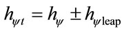 (24)
(24)
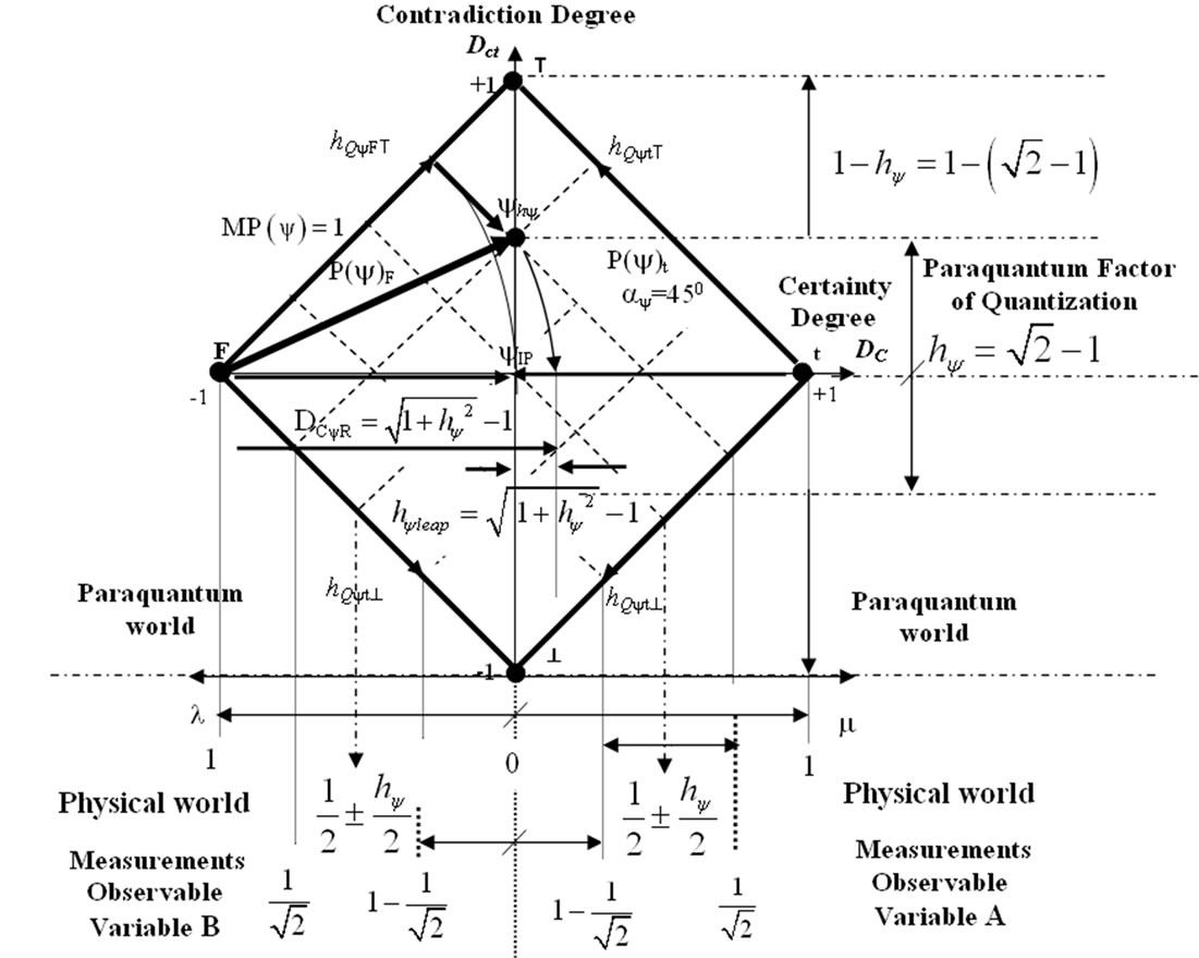
Figure 2. The paraquantum factor of quantization on the paraquantum logical state of quantization yhy due to paraquantum leap.
where from (22): .
.
Concerning the action of the Factor of Paraquantum Quantization hψ on the PQL Fundamental Lattice, we must also consider the effect of the Paraquantum Leap that produces quantities that will be either added or subtracted. So, the Factor of Paraquantum Quantization in its complete or total form which acts on the quantities is:
 (25)
(25)
Being:  the total Factor of Paraquantum Quantization at the time of arrival of the Superposed Paraquantum Logical state ψsup at the point where the Paraquantum Logical state of Quantization ψhψ is located.
 is the total Paraquantum Factor of Quantization at the departure of the Superposed Paraquantum Logical state ψsup at the point where the Paraquantum Logical state of Quantization ψhψ is located.
3.4. Newton Gamma Factor
In order to apply the Paraquantum Logics PQL in physical systems, it is important to study the Newton’s laws which relate the involved physical quantities (force, mass and acceleration) with the British System of units, as well as the implications that come up with the transformations to the International System of units (SI) (see [13]). The deductions of the second Newton’s Law indicate that if a resultant of forces acts on a body, this body receives an acceleration which is proportional to the force (F) and inversely proportional to its mass (m) (see [13, 14]). When it is mathematically expressed, this statement depends on a value that adjusts or establishes this proportionality between the quantities such that: 
or
 (26)
(26)
a is the acceleration or the ratio in which the body’s velocity changes through time.
F is the resultant of all forces which act on the body.
m is the body’s mass.
k is a proportionality adjustment factor.
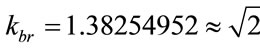
When we compare values between the quantities, we observe that for the International System of units (SI) to express the value of force F in a unit of Newton, an adjustment on the value of mass is necessary. Doing such comparisons and analogies between the unit Systems we obtain a unitary proportionality factor k of Equation (26)which expresses Newton’s second law, in the International System of units (SI). In order to adapt this framework to the PQL concepts, we have to multiply the proportionality adjustment factor kbr of the British System of units by 10 and divide the proportionality adjustment factor kSI of the International System of units (SI) by 10 (see [12]). Therefore:
 and
and .
.
We can adapt the proportionality factors k obtained for the Paraquantum Logical model as follows:
 and
and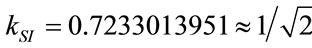 .
.
Given the importance of the Factor , which will be largely used in the equations of the PQL, its value is called Newton Gamma Factor whose symbol is
 . Therefore, in order to apply classical logics in the Paraquantum Logical model, the Newton Gamma Factor is
 .
.
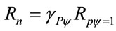
3.5. Paraquantum Gamma Factor γpψ
When we consider the Equation (23) just in the obtaining of favorable Evidence degree, it can be mathematically expressed through the multiplications between inversed values of the Newton Gamma Factor. For an expansion process where we consider quantizations based in consecutive applications of inversed values of the Newton Gamma Factor we can identify the Lorentz Factor γ in the infinite Power Series of the binomial expansion [13,14] related to the series obtained from consecutively applying the Newton Gamma Factor γN. In the paraquantum analysis we define a correlation value called Paraquantum Gamma Factor γpψ [12] such that:
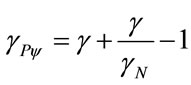 (27)
(27)
where:  is the Newton Gamma Factor:
 is the Lorentz factor which is:
Using the Paraquantum Gamma Factor  allows the computations, which correlate values of Observable Variables to the values related to quantization through the Paraquantum Quantization Factor hψ [11,12].
4. Paraquantum Logical Model Applied in Calculations of Quantization of Values of Physical Quantities
The quantitative analysis on the PQL Lattice defines a quantitative value QValor of any physical quantity, which can be represented on the horizontal axis of the certainty degrees and on the vertical axis of the contradiction degrees of the PQL Lattice. Since the maximum value is normalized on the PQL Fundamental Lattice [11], considering the Paraquantum Factor of quantization only, we can write: .
.
Doing so, the unitary value of the quantization is equivalent to a paraquantum quantization represented in the Paraquantum Logical state ψhψ added to the value of its complement. We have:
 (28)
(28)
where:  is the value of the total amount represented on the unitary axis of the PQL Fundamental Lattice.
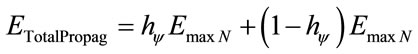
Equation (28) shows that the maximum amount of any quantity in the physical environment is composed by two quantized fractions where: one is determined on the Paraquantum Logical state of Quantization ψhψ by the Paraquantum Factor of Quantization hψ and the other is determined by its complement (1 – hψ). When the Paraquantum Gamma Factor  is applied on the paraquantum quantities, besides correlating the paraquantum values to the physical environment, it also works as a factor of expansion or contraction of the PQL Lattice.
4.1. Representation of Levels of Energy
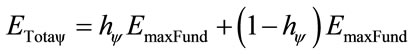
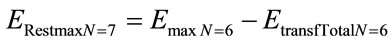
Consecutive applications of the Paraquantum Factor of Quantization hψ will produce Superposed Local Fundamental Lattices that will be related to the values of quantities in the physical environment [11,12]. When the values of quantities of the Equation (28) are related to energy, we can establish levels of energizing, creating Paraquantum models which act as mirrors of the systems in the physical environment. Figure 3 shows a Paraquantum Logical model where the Superposed Paraquantum Lattices are related in both the physical and Paraquantum environments and produce levels of energy which will be used to analyze the Hydrogen atom.
We observe that on Figure 3, the radius of the horizontal propagation of the Paraquantum logical states on the Fundamental Lattice can be computed. Since it is a value related to the Paraquantum Logical Model, this radius is determined through a Paraquantum quantity computed by: 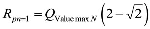
 (29)
(29)
4.2. Obtaining the Quantified Values in the Levels of Energy
By representing the involved Energy in the Paraconsistent Logical Model as being the energy amount represented on the vertical axis of contradiction, we can initially make an analogy with Equation (28) which defines the amount on the Fundamental Lattice in its static form. So, for the Energy, the equation is:
 (30)
(30)
When related to the physical environment, we have:
Figure 3. Model of the superposed local fundamental lattices where we can represent systems of energizing levels through the fundamental lattice.

Since that in the newtonian universe the value of velocity v related to the velocity of light c in the vacuum is too low, then the Factor of Lorentz is unitary:  and on Equation (27), the Paraquantum Gamma Factor computed with the Newton Factor
  is:
is: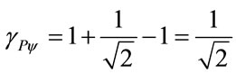 . In these conditions, the Paraquantum Gamma Factor
  is identical to the inverse value of the Newton Gamma Factor
 .
.
 (31)
(31)
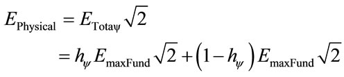
Being the total Energy: 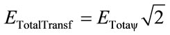
Then, doing: 
We can define the equation of the energy levels such that:
 (32)
(32)
where:  is the total Energy which can be transformed through propagation.
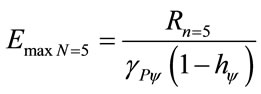
 is the maximum Energy on level N of the transition frequency.
N is the transition frequency or number of times of application of the Paraquantum Factor of Quantization.
We verify that, in the same way for quantities, the energy is quantized through the equilibrium point established by the Paraquantum Logical state of Quantization ψPψ [11,12].
4.3. The Quantified Values of the Levels of Energy in the Bohr Model
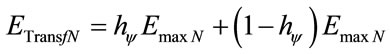
Based on Equation (32) the equation of the quantities of Energy, for the Bohr’s model on the Hydrogen atom [14,15], can be written as follows:
 (33)
(33)
where:
hψ is the Paraquantum Factor of quantization .
.
 is the total Energy that can be transformed through propagation, therefore through the orbit of the electron in the Hydrogen atom.
 is the maximum energy on the level N of transition frequency or in the current state of excitation of the electron.
N is the transition frequency or number of times of application of the Paraquantum Factor of Quantization.
We observe that on Bohr’s model, the value of N coincides with the excitation state of the electron.
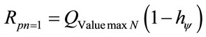
In the physical system composed by the atom, the first term of the Equation (33) is the quantity of energy of propagation that was transformed so that the electron reaches the equilibrium point its fundamental state. So, the value of the quantity of Energy of Propagation quantized, when considered in its static form, therefore, without considering the effect of the Paraquantum Leap, is computed by:
 (34)
(34)
where: hψ is the Paraquantum Factor of Quantization.
 is the Energy transformed in the propagation of the Paraquantum Logical state of the extreme Vertex False until it reaches the point where the Paraquantum Logical state of Quantization ψhψ is located.
 is the maximum Energy on the level N of the transition frequency or on the current state of excitation of the electron.
Since the process of transformation of energy is dynamical, we must consider the effects of Paraquantum Leaps on the Paraquantum Logical Model. So, the total energy transformed, that will constitute the Superposed Fundamental Lattice for the next level which will reach the electron, will be obtained with adding the Inertial or Irradiating Energy Eirr that appears due to the effects of Paraquantum Leaps.
Being the Factor of Quantization on the Paraquantum Leap defined on Equations (24) and (25), the Inertial or Irradiating Energy is expressed by:
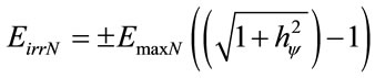 (35)
(35)
If Bohr’s Model [15] is used in the Paraquantum analysis, the electron will be considered a Paraquantum Logical state ψ–e that propagates orbiting the logical state proton ψ+Z located on the Paraquantum Logical state Undefined ψI. So, the positive or negative sign of the Equation (35) indicates if the analysis is at the arrival or at the departure of the electron at the equilibrium point where the Paraquantum Logical state of Quantization ψhψ is located. Since the electron, in the Model of Hydrogen Atom, reaches the excitation level at the arrival at the equilibrium point, then the sign will positive at the instant of the analysis, only. So, the total energy transformed at the equilibrium point of the Lattice of the PQL is computed by:
 (36)
(36)
or:
 (37)
(37)
So, Equation (33) is rewritten as follows:
 (38)
(38)
or as follows:
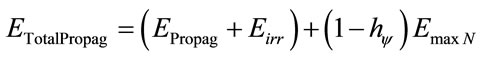 (39)
(39)
Or, in a more complete way, as follows:
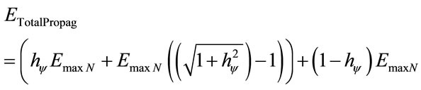 (40)
(40)
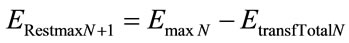
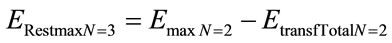
The second term of Equation (40) is the complemented value which represents the remaining maximum energy, therefore, it is that amount of energy capable of still being transformed in order to increase the excitation level of the electron. So, for each new excitation level of the electron, the remaining energy (ERestmax) is the one which outcomes the value which will be represented on the vertical and horizontal axis of the Lattice of the PQL.
For a static analysis, we have:
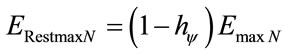 (41)
(41)
or
 (42)
(42)
Therefore, the remaining maximum Energy in the atom model depends on the excitation level of the electron. When the analysis process is considered dynamical, we must take the effect of the Paraquantum Leap into account and determine the Remaining maximum Energy adding the Inertial or Irradiating Energy. Then:
 (43)
(43)
or 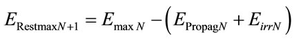
So, Equation (42) in its complete form is:
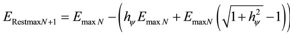 (44)
(44)
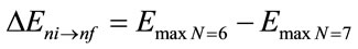
For variation of Energy between two levels:
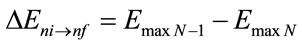 (45)
(45)
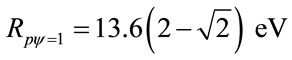
From Equation (28) we can compute the radius of horizontal propagation of the Paraquantum logical states on the Fundamental Lattice related to the values of amounts of the involved Energy [14]. So, the Horizontal Propagation Radius of Paraquantum propagation is computed by:
 (46)
(46)
As it was done for the Paraquantum values, this value obtained from the radius  can be related to the physical universe applying the Paraquantum Gamma Factor, that in the Newtonian universe is the inverse value of Newton Factor such that:
 (47)
(47)
If the value of the radius is known, we can determine the maximum value of energy on the level, such that:
 (48)
(48)
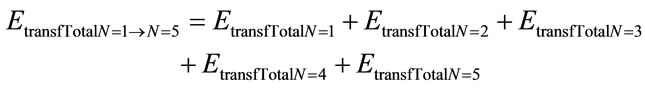
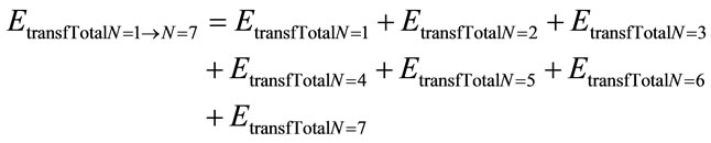
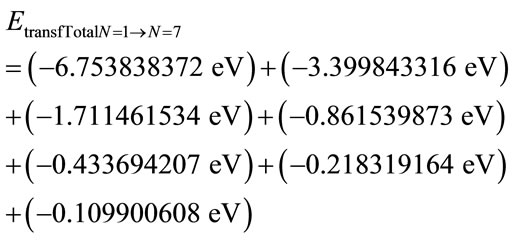
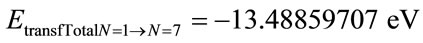
The energy transformed value between the Fundamental level n = 1 and the level n = N is:
 (49)
(49)
5. The Paraquantum Logic (PQL) Applied in the Atom of Hydrogen
For the application of the Paraquantum Logics PQL in the Hydrogen Atom we use, as a reference of values, the Bohr’s Model which describes an atom which has only an electron and one proton [14,15].
The idea in Bohr’s Model is the electrostatic attraction between the proton and the electron attracts the electron to the inner part of the atom and this force is compensated by the acceleration due to the circular movement of the electron [14]. About Bohr’s Model:
1) The force responsible for the cohesion of the atom is the Coulombian interaction between the electron and the core.
2) The core can be considered a fixed point.
3) The orbits of the electrons are circular.
4) The emission and absorption of radiation occur according to the Einstein’s assumption, that is, by the emission or absorption of a photon.
5.1. Conditions of Analyses of the Hydrogen Atom in Lattice of the PQL
Following the application methods of the PQL we will make a study that represents the Hydrogen atom on the Lattice of the PQL considering the results of the postulates of Bohr with the correlation features of the effects of propagation of the Paraquantum Logical states ψ and the bounding Factors of the Uncertainty Region of the PQL. So, the electron is considered a Superposed Paraquantum Logical state ψsup represented by ψ–el that propagates through the Fundamental Lattice of the PQL from the Vertex which represents the extreme Paraquantum Logical State False.
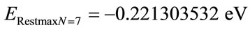
The propagation of the Paraquantum Logical state which represents the electron ψ–el is done around the Paraquantum Logical state Undefined ψI located on the equidistant point from the Vertices of the Fundamental Lattice where the Paraquantum Logical state of the proton represented by ψ+Z is located. So, according to the Paraquantum Logical model of the Hydrogen atom, the electron is a small Local Fundamental Lattice that propagates as a Paraquantum Logical state ψ-el and the proton is a minuscule fixed Local Fundamental Lattice represented at the equidistant point with the Paraquantum Logical state of Indefinition ψ+Z around which the electron orbits. Figure 4 shows the Lattice of PQL where the Hydrogen Atom is represented with the electron as a Paraquantum Logical state at the extreme Vertex of Falsity and the proton at the state of Pure Undefinition.
For constituting the Paraquantum Logical model based on Bohr’s model, the following assumptions are made for the Hydrogen atom that will be represented on the Fundamental Lattice of the PQL.
1) The electron that has charge –e will be represented by a Paraquantum logical state ψ–el.
2) The core composed by the Proton that has charge +Ze and will be represented by a Paraquantum logical state (ψ+Z) as a fixed point located equidistantly from the four vertices of the Lattice.
The orbit of the electron –e around the core +Ze in the atom that happens in the physical world is represented in the Paraquantum world through the propagation of the Paraquantum Logical state ψ–el. The electron orbiting the core in the physical world with its negative charge meets in its course electric and magnetic forces letting it in equilibrium in a certain level or state which can be the fundamental state or the n excited states.
Considering the initial condition where the Paraquantum Logical state ψ–el representing the electron is at the point located at the extreme Vertex False, its horizontal propagation represents the orbit of the electron in the physical world in the Fundamental state of Bohr’s model. So, on the Fundamental Lattice of the PQL, the Paraquantum logical state ψ–el will propagate crossing the vertical axis of the contradiction degrees at the Paraquantum Logical state of Quantization ψhψ. The propagation will be expressed through energy quantization determined by the Factor of Paraquantum Quantization hψ considering the Paraquantum Leaps through the variations on the value of the Real Certainty Degree that identifies the appearing of inertial or irradiating energy.
In the physical world, the insertion of energy into the
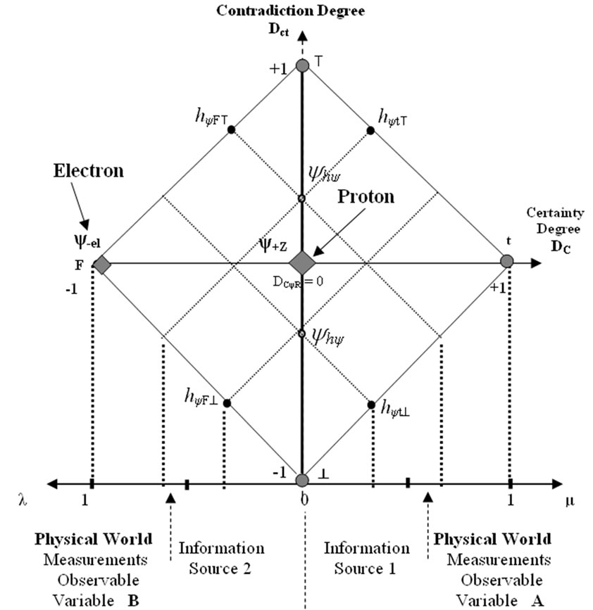
Figure 4. Representation of the hydrogen atom with the electron as a Paraquantum logical state at the extreme vertex of falsity and the proton at the state of pure undefinition.
atom causes disequilibrium and, if this disequilibrium is enough, it causes the electron to leave its fundamental state n = 1 and it makes the electron to reach another state of excitation. On the Fundamental Lattice of the PQL that represents the Hydrogen Atom, the Paraquantum logical state ψ–erel of the electron when propagating will transform the energy represented on the axis of the Certainty and Contradiction degrees and, for this, moves diagonally to one of the extreme Vertices of contradiction. When the Electron receives energy enough to reach another exciting state for n = 2, it means that the potential energy represented on the horizontal axis of the certainty degrees (EnDC) of the initial conditions is transformed in kinetic energy represented on the horizontal axis of the certainty degrees (EnDct) and reached enough to take it up, through two transitions to the excited level at the point where the Paraquantum Logical state of Quantization ψhψ is located. Figure 5 shows the propagation of the electron around the proton on the fundamental state n = 1.
This change of the electron from a state to another is done on the Paraquantum Logical model through the characteristics of the correlation that implies in considering the effects in the physical environment reflected on the Paraquantum world. So, all the equations we have studied about the Paraquantum effects are valid and correlated through the Paraquantum Factor of Quantization hψ for a Paraquantum model of the Hydrogen atom based on Bohr’s theories [15].
5.2. Comparative Study in the Application of the Paraquantum Logic (PQL) in the Hydrogen Atom
The correlation characteristics of the Relativistic Paraquantum Lattice and the transience property of the Superposed Paraquantum Logical states ψsup which propagate on the Fundamental Lattice of the PQL provide us with several conditions to make a comparative study of the Hydrogen atom using Bohr’s model. This study can be made directly with the energy levels of the Paraquantum correlation states through the equation that deals with quantities. So, each time that there is an increase of Energy defined by the Paraquantum Factor of Quantization hψ, there will be two transitions of the electron that will make it perform an orbit of a level of excited state in the Hydrogen atom. At the end of these two transitions of the electron, represented by the Paraquantum Logical state ψ–el, it will be on the equilibrium point of the Paraquantum Logical state of Quantization ψhψ. The energy on this point is determined by the addition of the energy transformed in the propagation Etporp with the Inertial of Irradiant Eirr which appears due to the Paraquantum Leaps.
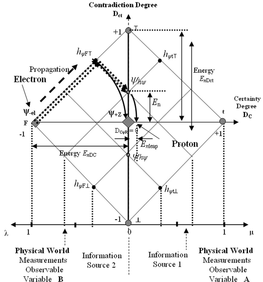
Figure 5. First propagation of the Paraquantum logical state ψ–el which represents the electron at the fundamental state n = 1 passes by the Paraquantum logical state of quantization ψhψ with the energy being quantized by the Paraquantum factor of quantization hψ.
5.3. The Spectrum of Radiation
Atomic spectra—which is the characteristic radiation emitted by the atoms of elements when they are heated, or submitted to electrical discharges—were studied at the end of the XIX century [14]. When observed with a spectroscopy, the radiation shows as a series of lines with different wave lengths, not always on a visible spectrum. Among many scientists that studied the atomic spectra, J.R. Rydberg and W. Ritz determined an empirical expression capable of compute the sequence of these lines. This expression is known as the Rydberg-Ritz formula and is given by [15]:
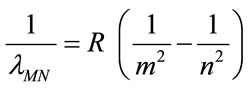 for n > m (50)
where: m and n are integers and R is the Rydberg constant, with result expressed in meters.
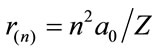
For Hydrogen, the value of R is 1.096776 × 10⁷ m–1 approaching a limit value of 1.097373 × 10⁷ m–1 for heavy elements [14]. This empirical expression can preview lines that are out of the range of the visible spectrum and have not been observed yet. According to the Bohr’s Postulate, the angular momentum of the electron is quantized and it is an integer number (n): . Comparing to its corresponding in the classical mechanics (L = mrv), we can find and define the value of r in function of n. So, we have:
 (51)
(51)
with 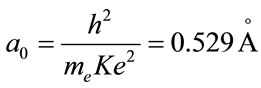
where: a0 is the constant called radius of Bohr.
By determining the expression of rn, we can find the expression of total Energy (En of the electron).
The equation of total Energy is expressed by:
 (52)
(52)
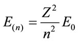
with .
.
We verify in this equation that En appears with a multiple of E0, whose value can be found and corresponds to 2.18 × 10⁻¹⁸ J or 13.6 eV.
According to Bohr’s postulate, the energy for an electronic transition, according to the set of allowed energies Em from position ni to position nf, is defined by:
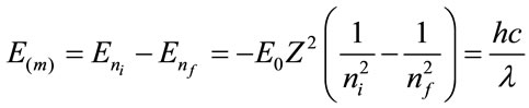 (53)
(53)
This value is the inverse of the wave length and Bohr compared it with the Rydberg-Ritz Formula, obtaining the theoretical value of the Rydberg’s constant which is equal to: . This results a value of R according to the experimental value.
Generally, the equations on Bohr’s model are featured with an integer number n which identifies the allowed orbits of the electron such that the electron can have orbits whose radiuses are 1, 4, 9, 16,  times the Bohr’s radius a0. On each allowed orbit, the electron is on a state with an energy which is constant and well defined with the following values:
Fundamental state n =1.
En(1) = –13.6 eV orbit with minimum radius r = aoExcited state n = 2 En(2) = –3.4 eVEm(2) = –10.2 eV orbit of radius r = 4aoExcited state n = 3 En(3) = –1.51 eVEm(3) = –12.09 eV orbit of radius r = 9aoExcited state n = 4 En(4) = –0.85 eVEm(4) = –12.75 eV orbit of radius r = 16aoExcited state n = 5 En(5) = –0.544 eVEm(5) = –13.06 eV orbit of radius r = 25aoExcited state n = 6 En(6) = –0.3777 eVEm(6) = –13.23 eV orbit of radius r = 36aoExcited state n = 7 En(7) = –0.27755 eVEm(7) = –13.32 eV orbit of radius r = 49ao.
5.4. Numerical Essay of the Levels of Energy through the Paraquantum Equations
Through the Paraquantum equations and the interpretation on the Lattice of the PQL, from where we obtain the energy levels with consecutive applications of the correlation factors, we can compute the values found on Bohr’s model for the Hydrogen atom. In this essay, we use the equations of the PQL for computing the values of energy quantities on excitation levels of the electron the Hydrogen atom.
● For the fundamental state n = 1.
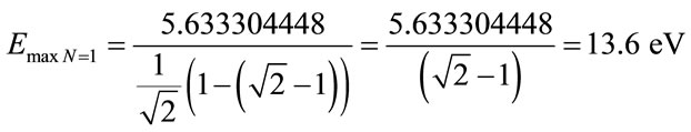
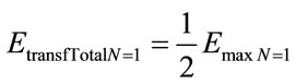
Initially, we have, on the fundamental state, the value that generates the Fundamental Lattice of the PQL for the Paraquantum Logical Model as being the value of Energy obtained by the Bohr’s equations.
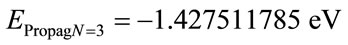
Using the value of the Energy obtained by the Bohr’s Equation (52), such that the Total Energy of the electron is: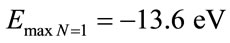 .
.
Through Paraquantum Equation (34) we can compute the Propagation Energy of the electron when it propagates through the Fundamental state.
 →
→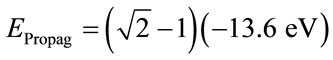
→
According to the Paraquantum Logical Model, the propagation of the electron is done on the edges of the Uncertainty Region of the Lattice of the PQL, so when it crosses the Vertical axis of the contradiction degrees on the point where the Paraquantum Logical state of Quantization ψhψ is located, we have the Inertial or Irradiant Energy caused by the Paraquantum Leap.
The Inertial or Irradiant Energy for the Fundamental level is computed by Equation (35) such that:

→
→
With Equation (36), the total transformed Energy for the Fundamental level is computed by:

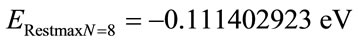
Through Equation (44) for the Fundamental level of excitation n = 1, we have the Remaining Energy to be transformed and it is computed by:


→
The Remaining Energy will be the Total Energy of the electron that will constitute the second Lattice of the PQL for the representation of the propagation of the electron at the excitation level n = 2.
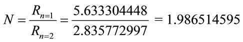
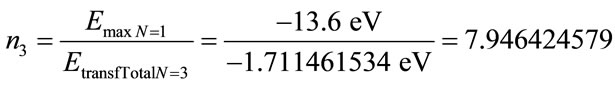
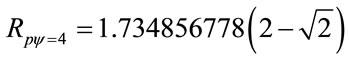
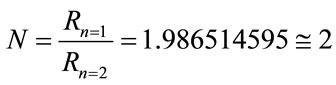
The value of the relation between the Total Energy of the electron of the Fundamental level n = 1 with the total transformed Energy of the same excitation state of the electron n = 1, is computed by:
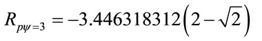
Equation (46) allows us to compute the Paraquantum absolute value of the Horizontal Propagation Radius for this level such that: 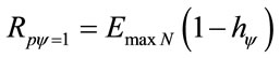
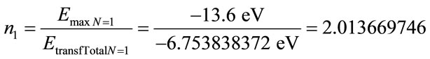
 →
→
→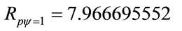
Using Equation (47), we compute the absolute value of the radius of Horizontal Propagation referring to the physical environment:

→ as
as 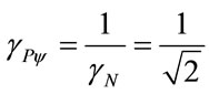
→
Equation (48) allows us to compute the maximum value of energy of the Fundamental level n = 1, such that:

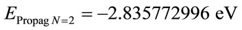
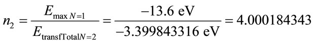
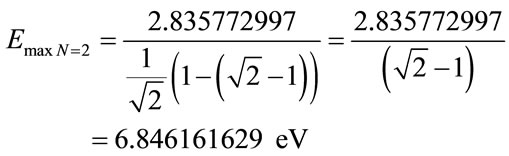
● For the excited state n = 2 the Total Energy of the electron is:
 .
.
And the variation of energy is computed by Equation (45):


→ .
.
By Equation (34) we have the Propagation Energy at the second excitation state of the electron n = 2 computed by: 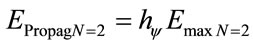

→ .
.
With Equation (35) the Inertial or Irradiant Energy for the level of the second excitement state of the electron n = 2 computed by:

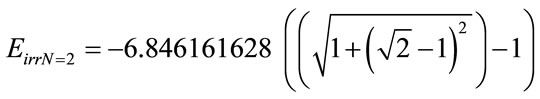
→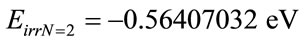 .
.
By Equation (36) the total transformed Energy to the level of the second excitement state of the electron n = 2 is computed by: 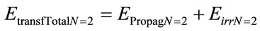

→ .
.
Through Equation (43) for the second level of excitation n = 3, we have the Remaining Energy to be transformed and it is computed by:

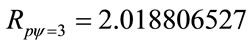
→
We can find the relation between the Total Energy of the electron of the Fundamental level n = 1 and the total transformed Energy of the level of the second excitement state of the electron n = 2 by doing:
By Equation (46) we can compute the Paraquantum absolute value of the Horizontal Propagation Radius for this level such that:
 →
→
By Equation (47) we compute the absolute value of the Horizontal Propagation radius that refers to the physical environment:
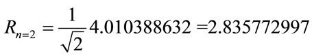
We can find the relation between the absolute value of the Horizontal Propagation radius that refers to the level of the second excitement state n = 2 and the Fundamental level n = 1:
Equation (48) allows us to compute the maximum energy value of the level of the second excitement state of the electron N = 2, such that:

By Equation (49) we compute the energy transformed value between the Fundamental level n = 1 and the level of the second excitement state of the electron n = 2, such that:


● For the excited state n = 3 the Total Energy of the electron is:
 .
.
And the variation of energy is computed by Equation (45): 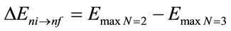

→
By Equation (34) we have: 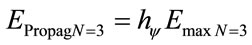
→
With Equation (35) the Inertial or Irradiant Energy for the level of the third excitement state of the electron n = 3 computed by:
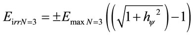

→
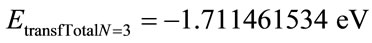
By Equation (36) the total transformed Energy to the level of the third excitement state of the electron n = 3 is computed by:
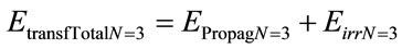

→
Through Equation (43) for the third level of excitation n = 3, we have the Remaining Energy to be transformed and it is computed by: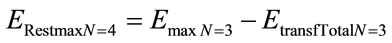

→
We can find the relation between the Total Energy of the electron of the Fundamental level n = 1 and the total transformed Energy of the level of the third excitement state of the electron n = 3 by doing:
By Equation (46) we can compute the Paraquantum absolute value of the Horizontal Propagation Radius for this level such that: 
→
By Equation (47) we compute the absolute value of the Horizontal Propagation radius that refers to the physical environment: 
→
We can find the relation between the absolute value of the Horizontal Propagation radius that refers to the level of the third excitement state n = 3 and the Fundamental level n = 1:
Equation (48) allows us to compute the maximum energy value of the level of the third excitement state of the electron n = 3, such that:


By Equation (49) we compute the energy transformed value between the Fundamental level n = 1 and the level of the third excitement state of the electron n = 3, such that:


● For the excited state n = 4 the Total Energy of the electron is:
 .
.
And the variation of energy is computed by Equation (45): 

→ .
.
By Equation (34) we have the Propagation Energy at the fourth excitation state of the electron n = 4 computed by: 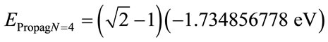
→ .
.
By Equation (35) the Inertial or Irradiant Energy for the level of the fourth excitement state of the electron n = 4 computed by:
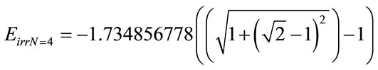
 .
.
The Total transformed energy to the level of the fourth Excitement state of the electron n = 4 is computed by:

→ .
.
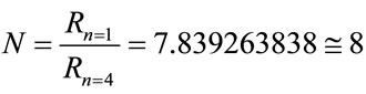
Through Equation (43) for the fourth level of excitation n = 4, we have the Remaining Energy to be transformed and it is computed by:


→ .
.
We can find the relation between the Total Energy of the electron of the Fundamental level n = 1 and the total transformed Energy of the level of the fourth excitement state of the electron n = 4 by doing:

By Equation (46) we can compute the Paraquantum absolute value of the Horizontal Propagation Radius for this level such that:
 →
→ .
.
By Equation (47) we compute the absolute value of the Horizontal Propagation radius that refers to the physical environment:
 .
.
We can find the relation between the absolute value of the Horizontal Propagation radius that refers to the level of the fourth excitement state n = 4 and the Fundamental level n = 1:
 .
.
Equation (48) allows us to compute the maximum energy value of the level of the fourth excitement state of the electron n = 4, such that:

By Equation (49) we compute the energy transformed value between the Fundamental level n = 1 and the level of the fourth excitement state of the electron n = 4, such that:

● For the excited state n = 5 the Total Energy of the electron is:
 .
.
And the variation of energy is computed by Equation (45): 

→
By Equation (34) we have the Propagation Energy at the fifth excitation state of the electron n = 5 computed by:

→
By Equation (35) the Inertial or Irradiant Energy for the level of the fifth excitement state of the electron n = 5 computed by:

The total transformed energy to the level of the fifth Excitement state of the electron n = 5 is computed by:


→
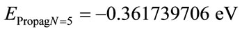
Through Equation (43) for the fifth level of excitation n = 5, we have the Remaining Energy to be transformed and it is computed by:

→
We can find the relation between the Total Energy of the electron of the Fundamental level n = 1 and the total transformed Energy of the level of the fifth excitement state of the electron n = 5 by doing:
By Equation (46) we can compute the Paraquantum absolute value of the Horizontal Propagation Radius for this level such that: 
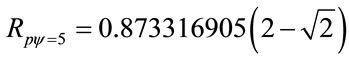 →
→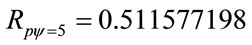
By Equation (47) we compute the absolute value of the Horizontal Propagation radius that refers to the physical environment:

We can find the relation between the absolute value of the Horizontal Propagation radius that refers to the level of the fifth excitement state n = 5 and the Fundamental level n = 1:

Equation (48) allows us to compute the maximum energy value of the level of the fifth excitement state of the electron n = 5, such that:

By Equation (49) we compute the energy transformed value between the Fundamental level n = 1 and the level of the fifth excitement state of the electron n = 5, such that:

● For the excited state n = 6 the Total Energy of the electron is:
 .
.
And the variation of energy is computed by Equation (45): 

→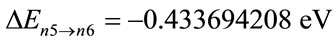
By Equation (34) we have the Propagation Energy at the sixth excitation state of the electron n = 6 computed by:

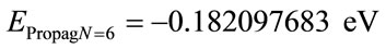
By Equation (35) the Inertial or Irradiant Energy for the level of the sixth excitement state of the electron n = 6 computed by:
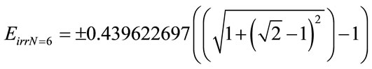
The Total transformed energy to the level of the sixth Excitement state of the electron n = 6 is computed by:


→
Through Equation (43) for the sixth level of excitation n = 6, we have the Remaining Energy to be transformed and it is computed by:

→
We can find the relation between the Total Energy of the electron of the Fundamental level n = 1 and the total transformed Energy of the level of the sixth excitement state of the electron n = 6 by doing:
By Equation (46) we can compute the Paraquantum absolute value of the Horizontal Propagation Radius for this level such that: 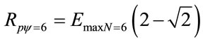
 →
→
By Equation (47) we compute the absolute value of the Horizontal Propagation radius that refers to the physical environment:
We can find the relation between the absolute value of the Horizontal Propagation radius that refers to the level of the sixth excitement state n = 6 and the Fundamental level n = 1:
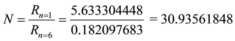
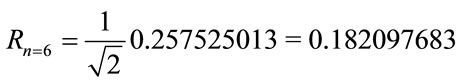
Equation (48) allows us to compute the maximum energy value of the level of the sixth excitement state of the electron n = 6, such that:

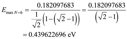
By Equation (49) we compute the energy transformed value between the Fundamental level n = 1 and the level of the sixth excitement state of the electron n = 6, such that:
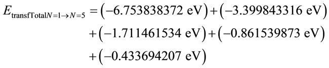
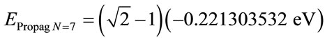
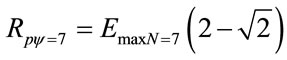
● For the excited state n = 7 the Total Energy of the electron is:

And the variation of energy is computed by Equation (45):

→
By Equation (34) we have the Propagation Energy at the seventh excitation state of the electron n = 7 computed by:
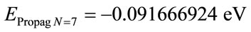
By Equation (35) the Inertial or Irradiant Energy for the level of the seventh excitement state of the electron n = 7 computed by:
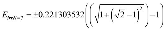

The total transformed energy to the level of the seventh Excitement state of the electron n = 7 is computed by:


→
Through Equation (43) for the seventh level of excitation n = 7, we have the Remaining Energy to be transformed and it is computed by:


→
We can find the relation between the Total Energy of the electron of the Fundamental level n = 1 and the total transformed Energy of the level of the seventh excitement state of the electron n = 7 by doing:

By Equation (46) we can compute the Paraquantum absolute value of the Horizontal Propagation Radius for this level such that:
 →
→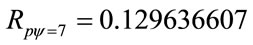
By Equation (47) we compute the absolute value of the Horizontal Propagation radius that refers to the physical environment:
We can find the relation between the absolute value of the Horizontal Propagation radius that refers to the level of the seventh excitement state n = 7 and the Fundamental level n = 1:
Equation (48) allows us to compute the maximum energy value of the level of the seventh excitement state of the electron n = 7, such that:

By Equation (49) we compute the energy transformed value between the Fundamental level n = 1 and the level of the seventh excitement state of the electron n = 7, such that:
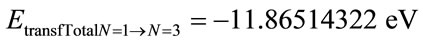
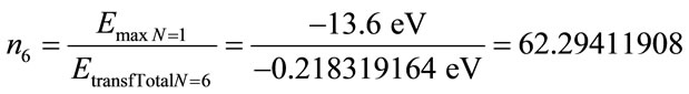
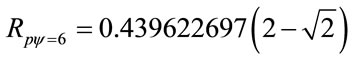
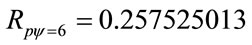
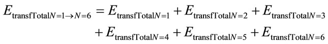
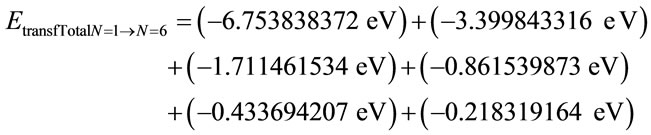
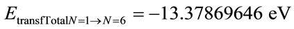
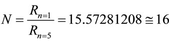
The values obtained through the Paraquantum equations for the Hydrogen atom model in 7 energy levels are showed on the Lattice of the PQL according to Figure 6 and Table 1.
5.5. Simplified Values
With the simplified values and with the possible rounding of the results, we can obtain the simplified equations used in the Bohr’s model.
For Level n = 1: 
→
For Level n = 2: 
→

For Level n = 3: 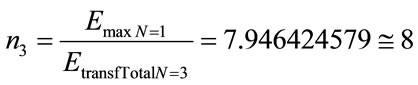
→

For Level n = 4: 
→

For Level n = 5: 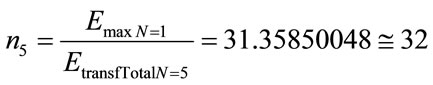
→
For Level n = 6: 
→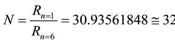

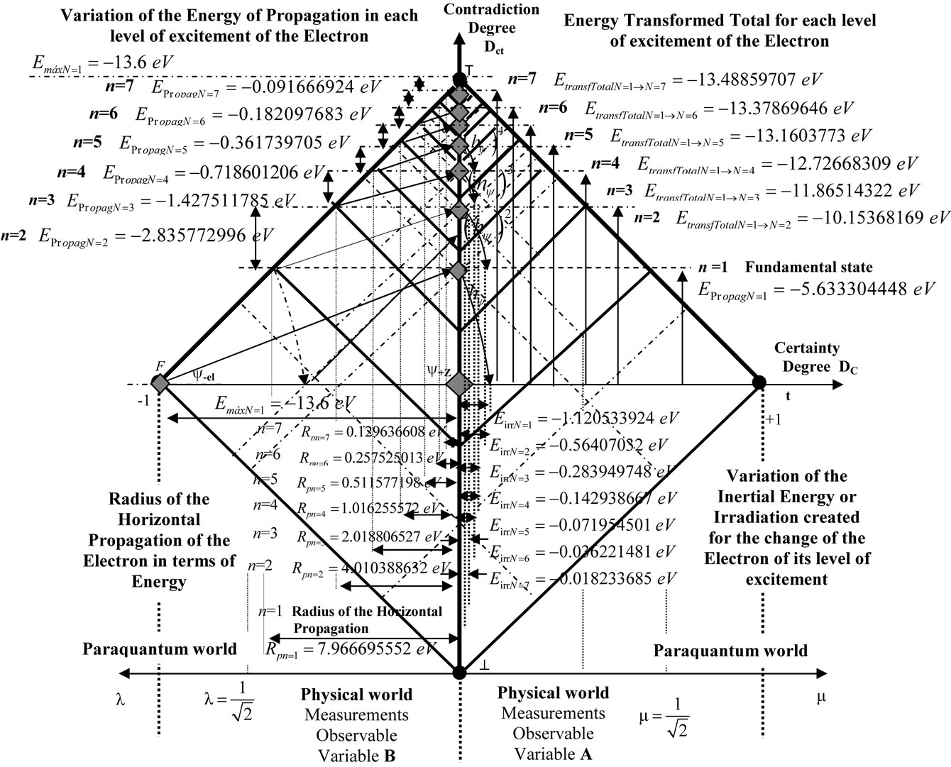
Figure 6. Values obtained by the equations when applying PQL to the hydrogen atom for seven energy levels.

Table 1. Comparative energy values between Paraquantum equations and Bohr’model.
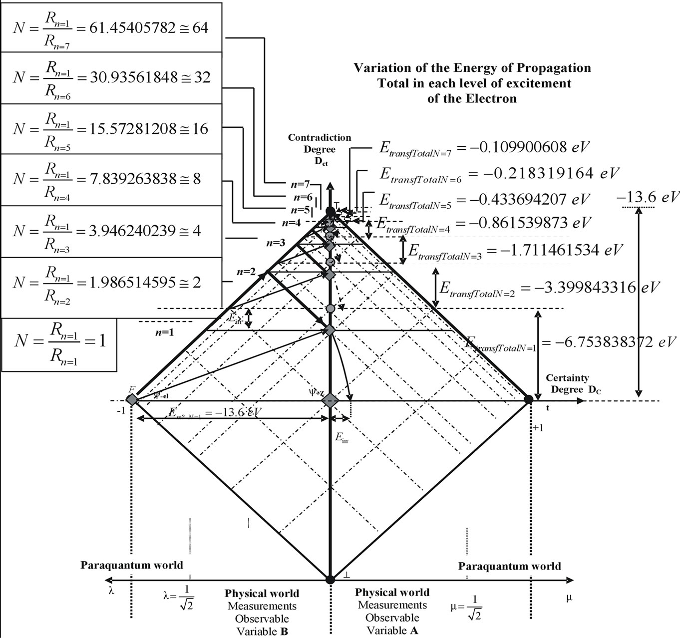
Figure 7. Simplified values obtained by the Paraquantum equations to the hydrogen atom for seven energy levels.
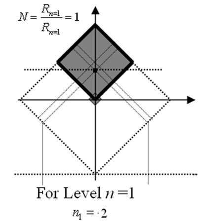

Figure 8. Simplified values and correlation with amount of lattices and electrons in each layer.
For Level n = 7: 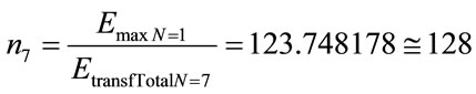
→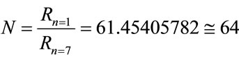

Figure 7 shows the results with simplified numeric values and Figure 8 shows the results with simplified values where the number of lattices in each level of energy can be considered as the amount of electrons capable of the atom to support in each layer.
The results obtained with the simplified values follow the equation: .
.
where: ne is the quantities of lattice or electrons and n is the atom level or energy layer.
6. Conclusions
In this paper we presented the main concepts of the PQLwith applications on physical Systems. The equations and forms of dealing with representative values of physical systems considered on the lattice of the PQL allowed to obtain behavioral characteristics of Paraquantum logical states ψ which produce quantitative results affected by the measurements performed on the Observable Variables in the physical environment. We presented the values which correlate the measurements of the evidence degrees in the physical environment with the quantization factors of the Paraquantum world. This correlation produced equations about physical quantities where through the Paraquantum equations we investigated the effects of energy balancing, quantization properties and transiences on the Paraquantum Logical Model in a comparative numerical study which deals with the PQL applied to the Bohr’s Model of the Hydrogen atom. The numerical results of the energy levels of the Hydrogen atom show that using the Paraquantum equations is a good option for modeling and solving questions related to the phenomena of physics. In the reference [16] we presented the Paraquantum Logical Model used in the calculations of the spectral analysis of the Hydrogen atom.
REFERENCES
- S. Jas’kowski, “Propositional Calculus for Contradictory Deductive Systems,” Studia Logica, Vol. 24, 1969, pp. 143-157. doi:10.1007/BF02134311
- N. C. A. Da Costa, “On the Theory of Inconsistent Formal Systems,” Notre Dame Journal of Formal Logic, Vol. 15, No. 4, 1974, pp. 497-510. doi:10.1305/ndjfl/1093891487
- N. C. A. Da Costa and D. Marconi, “An Overview of Paraconsistent Logic in the 80’s,” The Journal of NonClassical Logic, Vol. 6, No. 1, 1989, pp. 5-31.
- N. C. A. Da Costa, V. S. Subrahmaniane and C. Vago, “The Paraconsistent Logic PT,” Zeitschrift fur Mathematische Logik und Grundlagen der Mathematik, Vol. 37, 1991, pp. 139-148.
- J. I. Da Silva Filho, G. Lambert-Torres and J. M. Abe, “Uncertainty Treatment Using Paraconsistent Logic—Introducing Paraconsistent Artificial Neural Networks,” Vol. 21, IOS Press, Amsterdam, 2010, p. 328.
- J. I. Da Silva Filho, G. Lambert-Torres, L. F. P. Ferrara, A. M. C. Mário, M. R. Santos, A. S. Onuki, J. M. Camargo and A. Rocco, “Paraconsistent Algorithm Extractor of Contradiction Effects—Paraextrctr,” Journal of Software Engineering and Applications, Vol. 4, No. 10, 2011, pp. 579-584. doi:10.4236/jsea.2011.410067
- J. I. Da Silva Filho, A. Rocco, A. S. Onuki, L. F. P. Ferrara and J. M. Camargo, “Electric Power Systems Contingencies Analysis by Paraconsistent Logic Application,” The 14th International Conference on Intelligent System Applications to Power Systems, Kaohsiung, 5-8 November 2007, pp. 1-6.
- C. A. Fuchs and A. Peres, “Quantum Theory Needs No ‘Interpretation’,” Physics Today, Vol. 53, No. 3, 2000, pp. 70-71. doi:10.1063/1.883004
- D. Krause and O. Bueno, “Scientific Theories, Models, and the Semantic Approach,” Principia, Vol. 11, No. 2, 2007, pp. 187-201.
- J. A. Wheeler and H. Z. Wojciech (Eds.), “Quantum Theory and Measurement,” Princeton University Press, Princeton, 1983.
- J. I. Da Silva Filho, “Paraconsistent Annotated Logic in Analysis of Physical Systems: Introducing the Paraquantum Factor of Quantization hψ,” Journal of Modern Physics, Vol. 2, No. 11, 2011, pp. 1397-1409. doi:10.4236/jmp.2011.211172
- J. I. Da Silva Filho, “Paraconsistent Annotated Logic in Analysis of Physical Systems: Introducing the Paraquantum Gamma Factor γψ,” Journal of Modern Physics, Vol. 2, No. 12, 2011, pp. 1455-1469. doi:10.4236/jmp.2011.212180
- Pl. A. Tipler, “Physics,” Worth Publishers Inc., New York, 1976.
- Pl. A. Tipler and G. M. Tosca, “Physics for Scientists,” 6th Edition, W. H. Freeman and Company, New York, 2007.
- Pl. A. Tipler and R. A. Llewellyn, “Modern Physics,” 5th Edition, W. H. Freeman and Company, New York, 2007.
- J. I. Da Silva Filho, “Analysis of the Spectral Line Emissions of the Hydrogen Atom with Paraquantum Logic,” Journal of Modern Physics, Vol. 3 No. 3, 2012, pp. 233- 254. doi:10.4236/jmp.2012.33033