ABSTRACT

In this research article, we investigate the stability of a complex dynamical system involving coupled rigid bodies consisting of three equal masses joined by three rigid rods of equal lengths, hinged at each of their bases. The system is free to oscillate in the vertical plane. We obtained the equation of motion using the generalized coordinates and the Euler-Lagrange equations. We then proceeded to study the stability of the dynamical systems using the Jacobian linearization method and subsequently confirmed our result by phase portrait analysis. Finally, we performed MathCAD simulation of the resulting ordinary differential equations, describing the dynamics of the system and obtained the graphical profiles for each generalized coordinates representing the angles measured with respect to the vertical axis. It is discovered that the coupled rigid pendulum gives rise to irregular oscillations with ever increasing amplitude. Furthermore, the resulting phase portrait analysis depicted spiral sources for each of the oscillating masses showing that the system under investigation is unstable.

Keywords:

Coupled Rigid Body, Differential Equations, Stability, Phase Portrait, MathCAD Simulation

1. Introduction

The dynamics of coupled bodies and oscillators is significant in mechanics, engineering, electronics as well as biological systems. They are mostly represented as nonlinear dynamical systems [1] . One of the most important stages in the analysis of any mechanical model is to establish and find the solution of the dynamical equations which are referred to as equations of motion [2] . The equations of motion are often derived by the Euler-Lagrange equations. The fundamental idea of the Lagrangean approach to mechanics is to reformulate the equations of motion in terms of the dynamical variables that describe the degree of freedom, and thereby incorporate constraint forces into the definition of the degrees of freedom rather than explicitly including them as forces in Newton’s second law. Of importance is the notion of stability of a given dynamical system, where we would be concerned with the stability of some critical point of the system. Indeed stability plays a central role in system engineering, especially in the field of control system and automation, with regards to both dynamics and control.

Chutiphon [3] suggested Lyapunov stability as a general and useful approach to analyze the stability of nonlinear systems. It has two approaches: indirect and direct methods. For the second method of Lyapunov (indirect method), the idea of system linearization around a given point is used and local stability within small stability regions is possibly achieved. Seyrania and Wang [4] studied the stability of periodic solutions of the harmonically excited Duffing’s equation with the direct application of the Lyapunov theorem. The damping coefficient and excitation amplitude are assumed to be small. The approximate methods were used to find the periodic solutions. They derived the stability conditions and found stable and unstable region on the frequency response curve.

Maliki and Nwoba [5] studied a mathematical model of a coupled system of harmonic oscillators using the generalized coordinates and Euler-Lagrange equation. Laplace transform was also used to get the analytical solution of the system. The stability analysis of the system was investigated by the direct method and it was observed that the coupled system is asymptotically stable for the strictly negative roots and strongly unstable for the positive roots.

Maliki and Okereke [6] investigated the stability analysis of certain third order linear and nonlinear ordinary differential equations. They employed the method of phase portrait analysis and showed, using simulation that the Hartman-Groβman theorem is verified, for a second order linearized system, which approximates the nonlinear system, preserving the topological features.

1.1. Statement of the Problem

We consider the problem of analyzing the dynamics of a triple pendulum as shown in Figure 1. Despite the complexity of the system we will obtain, with the help of the Euler Lagrange (E-L) equations, the equation of motion of each of the individual masses (assumed to be equal). The system is coupled and joined by three rigid rods of equal lengths, hinged to each of the masses.

1.2. Model Formulation

From the figure below we choose ${\theta }_1,{\theta }_2$ and ${\theta }_3$ as our generalized coordinates.

To compute the Lagrangean of the system, we first compute the total kinetic energy (K.E) and potential energy (P.E) of the system. However, we require the following expressions.

$x_1=l_1\sin {\theta }_1$ (1)

$y_1=-l_1\cos {\theta }_1$ (2)

$x_2=l_1\sin {\theta }_1+l_2\sin {\theta }_2$ (3)

$y_2=-l_1\cos {\theta }_1-l_2\cos {\theta }_2$ (4)

$x_3=l_1\sin {\theta }_1+l_2\sin {\theta }_2+l_3\sin {\theta }_3$ (5)

$y_3=-l_1\cos {\theta }_1-l_2\cos {\theta }_2-l_3\cos {\theta }_3$ (6)

Differentiating the above coordinates with respect to time, we get;

${\dot{x}}_1=l_1{\dot{\theta }}_1\cos {\theta }_1$ (7)

${\dot{y}}_1=l_1{\dot{\theta }}_1\sin {\theta }_1$ (8)

${\dot{x}}_2=l_1{\dot{\theta }}_1\cos {\theta }_1+l_2{\dot{\theta }}_2\cos {\theta }_2$ (9)

${\dot{y}}_2=l_1{\dot{\theta }}_1\sin {\theta }_1+l_2{\dot{\theta }}_2\sin {\theta }_2$ (10)

${\dot{x}}_3=l_1{\dot{\theta }}_1\cos {\theta }_1+l_2{\dot{\theta }}_2\cos {\theta }_2+l_3{\dot{\theta }}_3\cos {\theta }_3$ (11)

${\dot{y}}_3=l_1{\dot{\theta }}_1\sin {\theta }_1+l_2{\dot{\theta }}_2\sin {\theta }_2+l_3{\dot{\theta }}_3\sin {\theta }_3$ (12)

The square of the velocities for each mass is given by;

$v_1^2={\dot{x}}^2{}_1+{\dot{y}}^2{}_1={\left(l_1{\dot{\theta }}_1\cos {\theta }_1\right)}^2+{\left(l_1{\dot{\theta }}_1\sin {\theta }_1\right)}^2=l_1^2{\dot{\theta }}^2{}_1$ (13)

Similarly,

$\begin{array}{c}{v}_2^2={\dot{x}}^2{}_2+{\dot{y}}^2{}_2={\left(l_1{\dot{\theta }}_1\cos {\theta }_1+l_2{\dot{\theta }}_2\cos {\theta }_2\right)}^2+{\left(l_1{\dot{\theta }}_1\sin {\theta }_1+l_2{\dot{\theta }}_2\sin {\theta }_2\right)}^2\\ =l_1^2{\dot{\theta }}^2{}_1+l_2^2{\dot{\theta }}^2{}_2+2l_1{l}_2{\dot{\theta }}_1{\dot{\theta }}_2\cos \left({\theta }_1-{\theta }_2\right)\end{array}$ (14)

Finally,

$\begin{array}{l}{v}_3^2={\dot{x}}^2{}_3+{\dot{y}}^2{}_3={\left(l_1{\dot{\theta }}_1\cos {\theta }_1+l_2{\dot{\theta }}_2\cos {\theta }_2+l_3{\dot{\theta }}_3\cos {\theta }_3\right)}^2\\ +{\left(l_1{\dot{\theta }}_1\sin {\theta }_1+l_2{\dot{\theta }}_2\sin {\theta }_2+l_3{\dot{\theta }}_3\sin {\theta }_3\right)}^2\end{array}$

After some algebraic manipulations, we get

$\begin{array}{l}{v}_3^2=l_1^2{\dot{\theta }}^2{}_1+l_2^2{\dot{\theta }}^2{}_2+l_3^2{\dot{\theta }}^2{}_3+2[l_1{l}_2{\dot{\theta }}_1{\dot{\theta }}_2\text{cos}\left({\theta }_1-{\theta }_2\right)\\ +l_1{l}_3{\dot{\theta }}_1{\dot{\theta }}_3\cos \left({\theta }_1-{\theta }_3\right)+l_2{l}_3{\dot{\theta }}_2{\dot{\theta }}_3\cos \left({\theta }_2-{\theta }_3\right)]\end{array}$ (15)

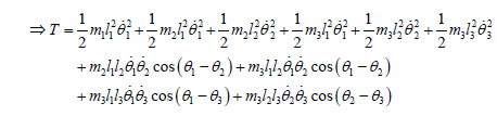
The total kinetic energy of the pendulum is then:

$\begin{array}{c}T=\frac{1}{2}{m}_1{v}_1^2+\frac{1}{2}{m}_2{v}_2^2+\frac{1}{2}{m}_3{v}_3^2\\ =\frac{1}{2}{m}_1{l}_1^2{\dot{\theta }}^2{}_1+\frac{1}{2}{m}_2\left[l_1^2{\dot{\theta }}^2{}_1+l_2^2{\dot{\theta }}^2{}_2+2l_1{l}_2{\dot{\theta }}_1{\dot{\theta }}_2\cos \left({\theta }_1-{\theta }_2\right)\right]\\ +\frac{1}{2}{m}_3(l_1^2{\dot{\theta }}^2{}_1+l_2^2{\dot{\theta }}^2{}_2+l_3^2{\dot{\theta }}^2{}_3+2[l_1{l}_2{\dot{\theta }}_1{\dot{\theta }}_2\cos \left({\theta }_1-{\theta }_2\right)\\ +l_1{l}_3{\dot{\theta }}_1{\dot{\theta }}_3\cos \left({\theta }_1-{\theta }_3\right)+l_2{l}_3{\dot{\theta }}_2{\dot{\theta }}_3\cos \left({\theta }_2-{\theta }_3\right)])\end{array}$ (16)

(17)

The total potential energy of the pendulum is the sum of the potential energy of each mass;

$V=m_{1}g{y}_1+m_{2}g{y}_2+m_{3}g{y}_3$

$\begin{array}{l}\Rightarrow V=-m_{1}g{l}_1\cos {\theta }_1+m_{2}g\left(-l_1\cos {\theta }_1-l_2\cos {\theta }_2\right)\\ +m_{3}g\left(-l_1\cos {\theta }_1-l_2\cos {\theta }_2-l_3\cos {\theta }_3\right)\end{array}$ (18)

Recall that the Lagrangean is given by $L=T-V$ .

$\begin{array}{l}\therefore L=\frac{1}{2}{m}_1{l}_1^2{\dot{\theta }}^2{}_1+\frac{1}{2}{m}_2{l}_1^2{\dot{\theta }}^2{}_1+\frac{1}{2}{m}_2{l}_2^2{\dot{\theta }}^2{}_2+\frac{1}{2}{m}_3{l}_1^2{\dot{\theta }}^2{}_1+\frac{1}{2}{m}_3{l}_2^2{\dot{\theta }}^2{}_2+\frac{1}{2}{m}_3{l}_3^2{\dot{\theta }}^2{}_3\\ +m_2{l}_1{l}_2{\dot{\theta }}_1{\dot{\theta }}_2\cos \left({\theta }_1-{\theta }_2\right)+m_3{l}_1{l}_2{\dot{\theta }}_1{\dot{\theta }}_2\cos \left({\theta }_1-{\theta }_2\right)+m_3{l}_1{l}_3{\dot{\theta }}_1{\dot{\theta }}_3\cos \left({\theta }_1-{\theta }_3\right)\\ +m_3{l}_2{l}_3{\dot{\theta }}_2{\dot{\theta }}_3\cos \left({\theta }_2-{\theta }_3\right)+m_{2}g{l}_1\cos {\theta }_1+m_{2}g{l}_2\cos {\theta }_2\\ +m_{3}g{l}_1\cos {\theta }_1+m_{3}g{l}_2\cos {\theta }_2+m_{3}g{l}_3\cos {\theta }_3\end{array}$ (19)

We now employ the E-L equations to obtain the equations of motion, i.e.;

$\frac{\text{d}}{\text{d}t}\left(\frac{\partial L}{\partial {\dot{\theta }}_j}\right)-\frac{\partial L}{\partial {\theta }_j}=0,j=1,2,3$ (20)

For the first generalized coordinate j = 1, we have;

$\begin{array}{l}\frac{\partial L}{\partial {\dot{\theta }}_1}=m_1{l}_1^2{\dot{\theta }}_1+m_2{l}_1^2{\dot{\theta }}_1+m_2{l}_1{l}_2{\dot{\theta }}_2\cos \left({\theta }_1-{\theta }_2\right)+m_3{l}_1^2{\dot{\theta }}_1\\ +m_3{l}_1{l}_2{\dot{\theta }}_2\cos \left({\theta }_1-{\theta }_2\right)+m_3{l}_1{l}_3{\dot{\theta }}_3\cos \left({\theta }_1-{\theta }_3\right)\end{array}$

$\begin{array}{l}\Rightarrow \frac{\partial L}{\partial {\dot{\theta }}_1}=l_1^2{\dot{\theta }}_1\left(m_1+m_2+m_3\right)+l_1{l}_2{\dot{\theta }}_2\left(m_2+m_3\right)\cos \left({\theta }_1-{\theta }_2\right)\\ +m_3{l}_1{l}_3{\dot{\theta }}_3\cos \left({\theta }_1-{\theta }_3\right)\end{array}$

$\begin{array}{l}\therefore \frac{\text{d}}{\text{d}t}\left(\frac{\partial L}{\partial {\dot{\theta }}_1}\right)=l_1^2{\ddot{\theta }}_1\left(m_1+m_2+m_3\right)+l_1{l}_2{\dot{\theta }}_2\left(m_2+m_3\right)\cos \left({\theta }_1-{\theta }_2\right)\\ +m_3{l}_1{l}_3{\dot{\theta }}_3\cos \left({\theta }_1-{\theta }_3\right)\end{array}$

Furthermore

$\begin{array}{l}\frac{\partial L}{\partial {\theta }_1}=-m_2{l}_1{l}_2{\dot{\theta }}_1{\dot{\theta }}_2\sin \left({\theta }_1-{\theta }_2\right)-m_3{l}_1{l}_2{\dot{\theta }}_1{\dot{\theta }}_2\sin \left({\theta }_1-{\theta }_2\right)-m_3{l}_1{l}_3{\dot{\theta }}_1{\dot{\theta }}_3\sin \left({\theta }_1-{\theta }_3\right)\\ -m_{1}g{l}_1\sin {\theta }_1-m_{2}g{l}_1\sin {\theta }_1-m_{3}g{l}_1\sin {\theta }_1\end{array}$

$\begin{array}{l}\Rightarrow \frac{\partial L}{\partial {\theta }_1}=-l_1{l}_2{\dot{\theta }}_1{\dot{\theta }}_2\left(m_2+m_3\right)\sin \left({\theta }_1-{\theta }_2\right)-m_3{l}_1{l}_3{\dot{\theta }}_1{\dot{\theta }}_3\sin \left({\theta }_1-{\theta }_3\right)\\ -g{l}_1\sin {\theta }_1\left(m_1+m_2+m_3\right)\end{array}$

$\begin{array}{l}\therefore \frac{\text{d}}{\text{d}t}\left(\frac{\partial L}{\partial {\dot{\theta }}_1}\right)-\frac{\partial L}{\partial {\theta }_1}=l_1^2{\ddot{\theta }}_1\left(m_1+m_2+m_3\right)+l_1{l}_2{\dot{\theta }}_2\left(m_2+m_3\right)\cos \left({\theta }_1-{\theta }_2\right)\\ +m_3{l}_1{l}_3{\dot{\theta }}_3\cos \left({\theta }_1-{\theta }_3\right)+l_1{l}_2{\dot{\theta }}_1{\dot{\theta }}_2\left(m_2+m_3\right)\sin \left({\theta }_1-{\theta }_2\right)\\ +m_3{l}_1{l}_3{\dot{\theta }}_1{\dot{\theta }}_3\sin \left({\theta }_1-{\theta }_3\right)+g{l}_1\sin {\theta }_1\left(m_1+m_2+m_3\right)=0\end{array}$ (21)

For the second generalized coordinate j = 2 in (1.20), we have;

$\begin{array}{c}\frac{\partial L}{\partial {\dot{\theta }}_2}=m_2{l}_2^2{\dot{\theta }}_2+m_2{l}_1{l}_2{\dot{\theta }}_1\cos \left({\theta }_1-{\theta }_2\right)+m_3{l}_2^2{\dot{\theta }}_2\\ +m_3{l}_1{l}_2{\dot{\theta }}_1\cos \left({\theta }_1-{\theta }_2\right)+m_3{l}_2{l}_3{\dot{\theta }}_3\cos \left({\theta }_2-{\theta }_3\right)\\ =l_2^2{\dot{\theta }}_2\left(m_2+m_3\right)+l_1{l}_2{\dot{\theta }}_1\left(m_2+m_3\right)\cos \left({\theta }_1-{\theta }_2\right)+m_3{l}_2{l}_3{\dot{\theta }}_3\cos \left({\theta }_2-{\theta }_3\right)\end{array}$

$\begin{array}{l}\Rightarrow \frac{\text{d}}{\text{d}t}\left(\frac{\partial L}{\partial {\dot{\theta }}_2}\right)=l_2^2{\ddot{\theta }}_2\left(m_2+m_3\right)+l_1{l}_2{\dot{\theta }}_1\left(m_2+m_3\right)\cos \left({\theta }_1-{\theta }_2\right)\\ +m_3{l}_2{l}_3{\dot{\theta }}_3\cos \left({\theta }_2-{\theta }_3\right)\end{array}$

Also,

$\begin{array}{l}\frac{\partial L}{\partial {\theta }_2}=-m_2{l}_1{l}_2{\dot{\theta }}_1{\dot{\theta }}_2\sin \left({\theta }_1-{\theta }_2\right)-m_3{l}_1{l}_2{\dot{\theta }}_1{\dot{\theta }}_2\sin \left({\theta }_1-{\theta }_2\right)\\ -m_3{l}_2{l}_3{\dot{\theta }}_2{\dot{\theta }}_3\sin \left({\theta }_2-{\theta }_3\right)-m_{2}g{l}_2\sin {\theta }_2-m_{2}g{l}_2\sin {\theta }_2\end{array}$

$\begin{array}{l}\Rightarrow \frac{\partial L}{\partial {\theta }_2}=-l_1{l}_2{\dot{\theta }}_1{\dot{\theta }}_2\left(m_2+m_3\right)\sin \left({\theta }_1-{\theta }_2\right)-m_3{l}_2{l}_3{\dot{\theta }}_2{\dot{\theta }}_3\sin \left({\theta }_2-{\theta }_3\right)\\ -g{l}_2\sin {\theta }_2\left(m_2+m_3\right)\end{array}$

$\begin{array}{l}\therefore \frac{\text{d}}{\text{d}t}\left(\frac{\partial L}{\partial {\dot{\theta }}_2}\right)-\frac{\partial L}{\partial {\theta }_2}=l_2^2{\ddot{\theta }}_2\left(m_2+m_3\right)+l_1{l}_2{\dot{\theta }}_1\left(m_2+m_3\right)\cos \left({\theta }_1-{\theta }_2\right)\\ +m_3{l}_2{l}_3{\dot{\theta }}_3\cos \left({\theta }_2-{\theta }_3\right)+l_1{l}_2{\dot{\theta }}_1{\dot{\theta }}_2\left(m_2+m_3\right)\sin \left({\theta }_1-{\theta }_2\right)\\ +m_3{l}_2{l}_3{\dot{\theta }}_2{\dot{\theta }}_3\sin \left({\theta }_2-{\theta }_3\right)+g{l}_2\sin {\theta }_2\left(m_2+m_3\right)=0\end{array}$ (22)

For the third generalized coordinate j = 3 in (20), we have;

$\frac{\partial L}{\partial {\dot{\theta }}_3}=m_3{l}_3^2{\dot{\theta }}_3+m_3{l}_1{l}_3{\dot{\theta }}_1\cos \left({\theta }_1-{\theta }_3\right)+m_3{l}_2{l}_3{\dot{\theta }}_2\cos \left({\theta }_2-{\theta }_3\right)$

$\Rightarrow \frac{\text{d}}{\text{d}t}\left(\frac{\partial L}{\partial {\dot{\theta }}_3}\right)=m_3{l}_3^2{\ddot{\theta }}_3+m_3{l}_1{l}_3{\dot{\theta }}_1\cos \left({\theta }_1-{\theta }_3\right)+m_3{l}_2{l}_3{\dot{\theta }}_2\cos \left({\theta }_2-{\theta }_3\right)$

Furthermore,

$\frac{\partial L}{\partial {\theta }_3}=-m_3{l}_1{l}_3{\dot{\theta }}_1{\dot{\theta }}_3\sin \left({\theta }_1-{\theta }_3\right)-m_3{l}_2{l}_3{\dot{\theta }}_2{\dot{\theta }}_3\sin \left({\theta }_2-{\theta }_3\right)-m_{3}g{l}_3\sin {\theta }_3$

$\begin{array}{l}\Rightarrow \frac{\text{d}}{\text{d}t}\left(\frac{\partial L}{\partial {\dot{\theta }}_3}\right)-\frac{\partial L}{\partial {\theta }_3}=m_3{l}_3^2{\ddot{\theta }}_3+m_3{l}_1{l}_3{\dot{\theta }}_1\cos \left({\theta }_1-{\theta }_3\right)+m_3{l}_2{l}_3{\dot{\theta }}_2\cos \left({\theta }_2-{\theta }_3\right)\\ +m_3{l}_1{l}_3{\dot{\theta }}_1{\dot{\theta }}_3\sin \left({\theta }_1-{\theta }_3\right)+m_3{l}_2{l}_3{\dot{\theta }}_2{\dot{\theta }}_3\sin \left({\theta }_2-{\theta }_3\right)\\ +m_{3}g{l}_3\sin {\theta }_3=0\end{array}$ (23)

Therefore, the equations of motion are;

$\begin{array}{l}{l}_1^2{\ddot{\theta }}_1\left(m_1+m_2+m_3\right)+l_1{l}_2{\dot{\theta }}_2\left(m_2+m_3\right)\cos \left({\theta }_1-{\theta }_2\right)\\ +m_3{l}_1{l}_3{\dot{\theta }}_3\cos \left({\theta }_1-{\theta }_3\right)+l_1{l}_2{\dot{\theta }}_1{\dot{\theta }}_2\left(m_2+m_3\right)\sin \left({\theta }_1-{\theta }_2\right)\\ +m_3{l}_1{l}_3{\dot{\theta }}_1{\dot{\theta }}_3\sin \left({\theta }_1-{\theta }_3\right)+g{l}_1\left(m_1+m_2+m_3\right)\sin {\theta }_1=0\end{array}$ (24)

$\begin{array}{l}{l}_2^2{\ddot{\theta }}_2\left(m_2+m_3\right)+l_1{l}_2{\dot{\theta }}_1\left(m_2+m_3\right)\cos \left({\theta }_1-{\theta }_2\right)\\ +m_3{l}_2{l}_3{\dot{\theta }}_3\cos \left({\theta }_2-{\theta }_3\right)+l_1{l}_2{\dot{\theta }}_1^2\left(m_2+m_3\right)\sin \left({\theta }_1-{\theta }_2\right)\\ +m_3{l}_2{l}_3{\dot{\theta }}_2{\dot{\theta }}_3\sin \left({\theta }_2-{\theta }_3\right)+g{l}_2\left(m_2+m_3\right)\sin {\theta }_2=0\end{array}$ (25)

$\begin{array}{l}{m}_3{l}_3^2{\ddot{\theta }}_3+m_3{l}_1{l}_3{\dot{\theta }}_1\cos \left({\theta }_1-{\theta }_3\right)+m_3{l}_2{l}_3{\dot{\theta }}_2\cos \left({\theta }_2-{\theta }_3\right)\\ +m_3{l}_1{l}_3{\dot{\theta }}_1{\dot{\theta }}_3\sin \left({\theta }_1-{\theta }_3\right)+m_3{l}_2{l}_3{\dot{\theta }}_2{\dot{\theta }}_3\sin \left({\theta }_2-{\theta }_3\right)+m_{3}g{l}_3\sin {\theta }_3=0\end{array}$ (26)

Assuming equal masses and equal lengths of rods, i.e., $l_1=l_2=l_3=l$ , $m_1=m_2=m_3=m$ .

The equations become respectively;

$\begin{array}{l}3l^2{\ddot{\theta }}_{1}m+2l^2{\dot{\theta }}_{2}m\cos \left({\theta }_1-{\theta }_2\right)+m{l}^2{\dot{\theta }}_3\cos \left({\theta }_1-{\theta }_3\right)\\ +2l^2{\dot{\theta }}_1{\dot{\theta }}_{2}m\sin \left({\theta }_1-{\theta }_2\right)+m{l}^2{\dot{\theta }}_1{\dot{\theta }}_3\sin \left({\theta }_1-{\theta }_3\right)+3glm\sin {\theta }_1=0\end{array}$ (27)

$\begin{array}{l}2l^2{\ddot{\theta }}_{2}m+2l^2{\dot{\theta }}_{1}m\cos \left({\theta }_1-{\theta }_2\right)+m{l}^2{\dot{\theta }}_3\cos \left({\theta }_2-{\theta }_3\right)\\ +2l^2{\dot{\theta }}_1^{2}m\sin \left({\theta }_1-{\theta }_2\right)+m{l}^2{\dot{\theta }}_2{\dot{\theta }}_3\sin \left({\theta }_2-{\theta }_3\right)+2glm\sin {\theta }_2=0\end{array}$ (28)

$\begin{array}{l}m{l}^2{\ddot{\theta }}_3+m{l}^2{\dot{\theta }}_1\cos \left({\theta }_1-{\theta }_3\right)+m{l}^2{\dot{\theta }}_3\cos \left({\theta }_2-{\theta }_3\right)\\ +m{l}^2{\dot{\theta }}_1{\dot{\theta }}_3\sin \left({\theta }_1-{\theta }_3\right)+m{l}^2{\dot{\theta }}_2{\dot{\theta }}_3\sin \left({\theta }_2-{\theta }_3\right)+mgl\sin {\theta }_3=0\end{array}$ (29)

We assume the generalized coordinates ${\theta }_1,{\theta }_2,{\theta }_3$ representing the angular displacements are small so that;

$\sin {\theta }_i\approx {\theta }_i,sin\left({\theta }_i-{\theta }_j\right)\approx {\theta }_i-{\theta }_j,\cos \left({\theta }_i-{\theta }_j\right)\approx 1-\frac{1}{2}{\left({\theta }_i-{\theta }_j\right)}^2,\forall i\ne j$

The equations of motion for the coupled rigid body then become;

$\begin{array}{l}3{\ddot{\theta }}_1+2{\dot{\theta }}_2\left[1-\frac{1}{2}{\left({\theta }_1-{\theta }_2\right)}^2\right]+{\dot{\theta }}_3\left[1-\frac{1}{2}{\left({\theta }_1-{\theta }_3\right)}^2\right]\\ +2{\dot{\theta }}_1{\dot{\theta }}_2\left({\theta }_1-{\theta }_2\right)+{\dot{\theta }}_1{\dot{\theta }}_3\left({\theta }_1-{\theta }_3\right)+\frac{3g}{l}{\theta }_1=0\end{array}$

$\begin{array}{l}\Rightarrow 3{\ddot{\theta }}_1+2{\dot{\theta }}_2+{\dot{\theta }}_3-{\dot{\theta }}_2{\left({\theta }_1-{\theta }_2\right)}^2-\frac{1}{2}{\dot{\theta }}_3{\left({\theta }_1-{\theta }_3\right)}^2\\ +2{\dot{\theta }}_1{\dot{\theta }}_2\left({\theta }_1-{\theta }_2\right)+{\dot{\theta }}_1{\dot{\theta }}_3\left({\theta }_1-{\theta }_3\right)+\frac{3g}{l}{\theta }_1=0\end{array}$ (30)

Following the above procedure, we have for Equation (28)

$\begin{array}{l}2{\ddot{\theta }}_2+2{\dot{\theta }}_1\left[1-\frac{1}{2}{\left({\theta }_1-{\theta }_2\right)}^2\right]+{\dot{\theta }}_3\left[1-\frac{1}{2}{\left({\theta }_2-{\theta }_3\right)}^2\right]\\ +2{\dot{\theta }}_1^2\left({\theta }_1-{\theta }_2\right)+{\dot{\theta }}_2{\dot{\theta }}_3\left({\theta }_2-{\theta }_3\right)+\frac{2g}{l}{\theta }_2=0\end{array}$

$\begin{array}{l}\Rightarrow 2{\ddot{\theta }}_2+2{\dot{\theta }}_1+{\dot{\theta }}_3-\frac{1}{2}{\dot{\theta }}_1{\left({\theta }_1-{\theta }_2\right)}^2-\frac{1}{2}{\dot{\theta }}_3{\left({\theta }_2-{\theta }_3\right)}^2\\ +2{\dot{\theta }}_1^2\left({\theta }_1-{\theta }_2\right)+{\dot{\theta }}_2{\dot{\theta }}_3\left({\theta }_2-{\theta }_3\right)+\frac{2g}{l}{\theta }_2=0\end{array}$ (31)

Similarly for Equation (29) we have;

$\begin{array}{l}{\ddot{\theta }}_3+{\dot{\theta }}_1\left[1-\frac{1}{2}{\left({\theta }_1-{\theta }_3\right)}^2\right]+{\dot{\theta }}_3\left[1-\frac{1}{2}{\left({\theta }_2-{\theta }_3\right)}^2\right]\\ +{\dot{\theta }}_1{\dot{\theta }}_3\left({\theta }_1-{\theta }_3\right)+{\dot{\theta }}_2{\dot{\theta }}_3\left({\theta }_2-{\theta }_3\right)+\frac{g}{l}{\theta }_3=0\end{array}$

$\begin{array}{l}\Rightarrow {\ddot{\theta }}_3+{\dot{\theta }}_1+{\dot{\theta }}_3-\frac{1}{2}{\dot{\theta }}_1{\left({\theta }_1-{\theta }_3\right)}^2-\frac{1}{2}{\dot{\theta }}_3{\left({\theta }_2-{\theta }_3\right)}^2\\ +{\dot{\theta }}_1{\dot{\theta }}_3\left({\theta }_1-{\theta }_3\right)+{\dot{\theta }}_2{\dot{\theta }}_3\left({\theta }_2-{\theta }_3\right)+\frac{g}{l}{\theta }_3=0\end{array}$ (32)

The model equations for the given problem are summarized as;

$\{\begin{array}{l}{\ddot{\theta }}_1+\frac{2}{3}{\dot{\theta }}_2+\frac{1}{3}{\dot{\theta }}_3-\frac{1}{3}{\dot{\theta }}_2{\left({\theta }_1-{\theta }_2\right)}^2-\frac{1}{6}{\dot{\theta }}_3{\left({\theta }_1-{\theta }_3\right)}^2\\ +\frac{2}{3}{\dot{\theta }}_1{\dot{\theta }}_2\left({\theta }_1-{\theta }_2\right)+\frac{1}{3}{\dot{\theta }}_1{\dot{\theta }}_3\left({\theta }_1-{\theta }_3\right)+\frac{g}{l}{\theta }_1=0\\ {\ddot{\theta }}_2+{\dot{\theta }}_1+\frac{1}{2}{\dot{\theta }}_3-\frac{1}{4}{\dot{\theta }}_1{\left({\theta }_1-{\theta }_2\right)}^2-\frac{1}{4}{\dot{\theta }}_3{\left({\theta }_2-{\theta }_3\right)}^2\\ +{\dot{\theta }}_1^2\left({\theta }_1-{\theta }_2\right)+\frac{1}{2}{\dot{\theta }}_2{\dot{\theta }}_3\left({\theta }_2-{\theta }_3\right)+\frac{g}{l}{\theta }_2=0\\ {\ddot{\theta }}_3+{\dot{\theta }}_1+{\dot{\theta }}_3-\frac{1}{2}{\dot{\theta }}_1{\left({\theta }_1-{\theta }_3\right)}^2-\frac{1}{2}{\dot{\theta }}_3{\left({\theta }_2-{\theta }_3\right)}^2\\ +{\dot{\theta }}_1{\dot{\theta }}_3\left({\theta }_1-{\theta }_3\right)+{\dot{\theta }}_2{\dot{\theta }}_3\left({\theta }_2-{\theta }_3\right)+\frac{g}{l}{\theta }_3=0\end{array}$ (33)

1.3. Stability Analysis

For the purpose of stability analysis we must vectorize the above coupled system of differential equations.

Let $u_1={\theta }_1,u_2={\theta }_2,u_3={\theta }_3$ and ${\dot{u}}_1=u_4,{\dot{u}}_2=u_5,{\dot{u}}_3=u_6$ , hence ${\ddot{u}}_1={\dot{u}}_4,{\ddot{u}}_2={\dot{u}}_5,{\ddot{u}}_3={\dot{u}}_6$ Thus the vectorized system of equations for the coupled pendulums is;

${\dot{u}}_1=u_4$ (34)

${\dot{u}}_2=u_5$ (35)

${\dot{u}}_3=u_6$ (36)

$\begin{array}{l}{\dot{u}}_4=-\frac{2}{3}{u}_5-\frac{1}{3}{u}_6+\frac{1}{3}{u}_5{\left(u_1-u_2\right)}^2+\frac{2}{6}{u}_6{\left(u_1-u_3\right)}^2\\ -\frac{2}{3}{u}_4{u}_5\left(u_1-u_2\right)-\frac{1}{3}{u}_4{u}_6\left(u_1-u_3\right)-\frac{g}{l}{u}_1\end{array}$ (37)

$\begin{array}{l}{\dot{u}}_5=-u_4-\frac{1}{2}{u}_6+\frac{1}{4}{u}_4{\left(u_1-u_2\right)}^2+\frac{1}{4}{u}_6{\left(u_2-u_3\right)}^2\\ -u_4^2\left(u_1-u_2\right)-\frac{1}{2}{u}_5{u}_6\left(u_2-u_3\right)-\frac{g}{l}{u}_2\end{array}$ (38)

$\begin{array}{l}{\dot{u}}_6=-u_4-u_5+\frac{1}{2}{u}_4{\left(u_1-u_3\right)}^2+\frac{1}{2}{u}_6{\left(u_2-u_3\right)}^2\\ -u_4{u}_6\left(u_1-u_3\right)-u_5{u}_6\left(u_2-u_3\right)-\frac{g}{l}{u}_3\end{array}$ (39)

We shall investigate the stability of the pendulum at the critical point, where ${\dot{u}}_1={\dot{u}}_2={\dot{u}}_3={\dot{u}}_4={\dot{u}}_5={\dot{u}}_6=0$ . This implies that $u_4=0,u_5=0,u_6=0$ and by substitution our critical point is $\left(0,0,0,0,0,0\right)$ .

Equations (34)-(39) can, for convenience) be written simply as;

$\begin{array}{l}{\dot{u}}_1=f_1\left(u_1,\cdots ,u_6\right)\\ ⋮\\ {\dot{u}}_6=f_6\left(u_1,\cdots ,u_6\right)\end{array}$ (40)

where the $f_i\left(u_1,\cdots ,u_6\right),i=1,\cdots ,6$ represent the RHS of the system.

The Jacobian of the system is written

$J_f\left(u\right)={\left(\frac{\partial f_i}{\partial u_j}\right)}_{6\times 6}$ (41)

Computing the entries and evaluating at the critical point, we get

$J_f=\left(\begin{array}{cccccc}0& 0& 0& 1& 0& 0\\ 0& 0& 0& 0& 1& 0\\ 0& 0& 0& 0& 0& 1\\ -\frac{g}{l}& 0& 0& 0& -\frac{2}{3}& -\frac{1}{3}\\ 0& -\frac{g}{l}& 0& -1& 0& -\frac{1}{2}\\ 0& 0& -\frac{g}{l}& -1& -1& 0\end{array}\right)$

The eigenvalues of the matrix J are given by $\left|J_f-\lambda I\right|=0$ .

$\Rightarrow \left|\begin{array}{cccccc}-\lambda & 0& 0& 1& 0& 0\\ 0& -\lambda & 0& 0& 1& 0\\ 0& 0& -\lambda & 0& 0& 1\\ -\frac{g}{l}& 0& 0& -\lambda & -\frac{2}{3}& -\frac{1}{3}\\ 0& -\frac{g}{l}& 0& -1& -\lambda & -\frac{1}{2}\\ 0& 0& -\frac{g}{l}& -1& -1& -\lambda \end{array}\right|=0$

This simplifies to give;

${\lambda }^6+\left(-3\alpha -\frac{3}{2}\right){\lambda }^4+\frac{2}{3}{\lambda }^3+\left(3{\alpha }^2-\frac{3}{2}\alpha \right)\lambda -{\alpha }^3=0$ (42)

where $\alpha =-g/l$ . For simplicity we take $l=1$ , and naturally $g=9.8$ .

We now employ the POLYROOT algorithm in MathCad [7] to solve the polynomial Equation (42).

Define a vector v of the coefficients beginning with the constant term, i.e.:

$v={\left[\begin{array}{ccccccc}-{\alpha }^3& 0& \left(3{\alpha }^2+\frac{3}{2}\alpha \right)& \frac{2}{3}& \left(-3\alpha -\frac{3}{2}\right)& 0& 1\end{array}\right]}^{\text{T}}$ (43)

$\therefore \text{polyroots}\left(v\right)=\left[\begin{array}{c}-0.703-3.051i\\ -0.703+3.051i\\ 0.282+3.118i\\ \begin{array}{l}0.282-3.118i\\ 0.421-3.102i\\ 0.421+3.102i\end{array}\end{array}\right]$ (44)

Clearly not all the eigenvalues have negative real parts, we therefore conclude that the critical point of the system is unstable.

2. Simulation of the System of ODEs

In MathCAD we define the vector of derivatives, viz.;

Additional arguments for the ODE solver are

$t_0:=0$ Initial value of independent variable

$t_1:=10$ End value of independent variable

$Y_0:=\left(\begin{array}{c}0.01\\ 0\\ 0\\ 0\\ 0\\ 0\end{array}\right)$ Vector of initial function values

$num:=1\times {10}^3$ Number of solution values on [t₀, t₁]

Solution Matrix

$S1:=\text{Rkadapt}\left(Y_0,t_0,t_1,num,D\right)$

$t:=S{1}^{\langle 0\rangle }$ Independent variable values

$u_1:=S{1}^{\langle 1\rangle }$ First solution function values

$u_2:=S{1}^{\langle 2\rangle }$ Second solution function values

$u_3:=S{1}^{\langle 3\rangle }$ Third solution function values

$u_4:=S{1}^{\langle 4\rangle }$ Fourth solution function values

$u_5:=S{1}^{\langle 5\rangle }$ Fifth solution function values

$u_6:=S{1}^{\langle 6\rangle }$ Sixth solution function values

3. Discussion

Table 1 is the MathCad solution matrix for the system of differential equations describing the dynamics of the coupled pendulums. This solution matrix is obtained using the Runge-Kutta algorithm. Figures 2(a)-(c) depict the graphical profiles of the solution curves. We recall that the variables $u_1={\theta }_1,u_2={\theta }_2,u_3={\theta }_3$ are actually the generalized coordinates, representing the angular displacements from the vertical position, while their derivates with respect to time ${\dot{u}}_1=u_4,{\dot{u}}_2=u_5,{\dot{u}}_3=u_6$ are the angular velocities.

The graph of ${\theta }_1\left(t\right)$ (Figure 2(a)) starts from the origin, then performs irregular oscillations with increasing amplitude over time. Figure 2(b) and Figure 2(c) depict a similar variation for ${\theta }_2\left(t\right)$ and ${\theta }_3\left(t\right)$ .

Figure 2(g) is the profile of the combined graph of ${\theta }_1\left(t\right)$ , ${\theta }_2\left(t\right)$ and ${\theta }_3\left(t\right)$ against time. This is important because although the coupled pendulum performs irregular oscillations, at specific times the oscillations for each mass intersect, meaning they all pass through the same point. Furthermore, we observe that the respective amplitudes for each generalized coordinate is increasing. Figures 2(d)-(f) depict respectively the variation of the angular velocities

${\dot{\theta }}_1\left(t\right)=u_4$ , ${\dot{\theta }}_2\left(t\right)=u_5$ and ${\dot{\theta }}_3\left(t\right)=u_6$ . These velocities are clearly oscillatory and irregular with increasing amplitude.

Figures 3(a)-(c) are respectively the phase portrait for ${\dot{\theta }}_1\left(t\right)=u_4$ against ${\theta }_1\left(t\right)=u_1$ , ${\dot{\theta }}_2\left(t\right)=u_5$ against ${\theta }_2\left(t\right)=u_2$ and ${\dot{\theta }}_3\left(t\right)=u_6$ against ${\theta }_3\left(t\right)=u_3$ . For each of the phase portraits we obtain a spiral source.

4. Conclusions

Coupled oscillators in general, are useful in the study of vibrations and as such computing the specific modes of vibration for oscillating systems is very important from a practical point of view, particularly in engineering. The study of coupled systems is useful in mechanics, electronics as well as biological systems. It is also pertinent for the biomechanical analysis of animals, humans or robotic systems. An early application of mathematical modeling in biological systems was first pioneered by Van der Pol in 1928. The Van der Pol oscillator [8] was used to explain some normal and pathological rhythms of the heart.

Our research work has clearly demonstrated the power of mathematical modeling, where the behaviour of a complex mechanical system can be captured in the form of a system of ordinary differential equations. Furthermore, with versatile mathematical software such as MathCAD, the system can be analyzed in detailed graphical format to give a deep understanding of the inherent dynamics as well as its stability properties.

Cite this paper

Maliki, O.S. and Anozie, V.O. (2018) On the Stability Analysis of a Coupled Rigid Body. Applied Mathematics, 9, 210-222. https://doi.org/10.4236/am.2018.93016

References

- 1. Strogatz, S.H. (1994) Nonlinear Dynamics and Chaos: With Application to Physics, Biology, Chemistry and Engineering. Perseus Books Publishing, Cambridge.
- 2. Graciela, V.H. (2012) Dynamical Properties of a System of Heavy Lagrange Gyroscopes Formed in Closed Chain Applied in a Parallel System. Advanced Materials Research, 452-453, 507-510. https://doi.org/10.4028/http://www.scientific.net/AMR.452-453.507
- 3. Chutiphon, P. (2011) A Review of Fundamentals of Lyapunov Theory. The Journal of Applied Science, 10, 55-61.
- 4. Seyranian, A.P. and Wang, Y. (2011) On Stability of Periodic Solution of Duffing Equation. Journal of National Academy of Science of Armenia, 111(4).
- 5. Maliki, S.O. and Nwoba, P.O. (2014) Stability Analysis of a System of Coupled Harmonic Oscillators. Pelagia Research Library Advances in Applied Science Research, 5, 195-203.
- 6. Maliki, S.O. and Okereke, R.N. (2016) A Note on Differential Equation with a Large Parameter. Applied Mathematics, 7, 183-192. https://doi.org/10.4236/am.2016.73018
- 7. Mathcad Version 14. PTC (Parametric Technology Corporation) Software Products. http://communications@ptc.com
- 8. Verhulst, F. (1990) Nonlinear Differential Equations and Dynamical Systems. Springer-Verlag, New York. https://doi.org/10.1007/978-3-642-97149-5