ABSTRACT

In this paper, we investigate the existence of local limit cycles obtained by perturbing degenerate and weak foci of two-dimensional cubic systems of differential equations. In particular, we consider a specific class of such systems where the origin is a degenerate focus. By utilizing a Liapunov function method and the stability results that follow, we first determine constraints on the system to maximize the number of local limit cycles that can be obtained by perturbing the degenerate focus at the origin. Once this is established, we add on the additional assumption that the system has a weak focus at, where, and determine conditions to maximize the number of additional local limit cycles that can be obtained near this fixed point. We will ultimately achieve an example of a cubic system with three local limit cycles about the degenerate focus and one local limit cycle about the weak focus.

Keywords:

Planar Differential Equations, Local Limit Cycles, Degenerate Foci

1. Degenerate Focus

We begin our investigation of local limit cycles by considering a planar cubic system of the following form:

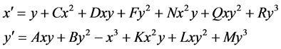(1)

where A, B, C, D, F, K, L, M, N, Q, and R are real constants. We note here that the origin is a degenerate focus as the linearization about the origin is nilpotent but nonzero, and the other necessary conditions, as given in Perko ( [1] , p. 173), are also met. To find local limit cycles of this system, we build a Liapunov function in the fashion outlined in Blows [2] , an extension of a result developed by Andreev, Sadovskii, and Tsikalyuk [3] . This function takes the form:

,

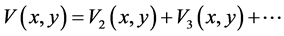where is homogeneous with degree m. By virtue of the chain rule, we see that:

.

For to be one-signed in a neighborhood of the origin, this implies that

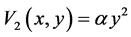
, for. We make the judicious choice of. Applying results

from Blows [2] , it follows that:

,

,

and so forth. These calculations quickly become tedious by hand, so the use of Mathe- matica, or a similar program capable of symbolic computation, is absolutely necessary to continue.

We are able to construct such that:

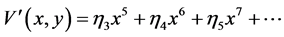
(see [2] ). Provided that the first nonzero value is of even degree, will be one-signed in a neighborhood of the origin and the stability of the degenerate focus is determined by its sign. If the first nonzero value is of odd degree, the method is inconclusive. If all values are zero, then we have a center. The set has a finite basis which we denote as. The L_i, called Liapunov numbers, are ordered as they arise in the construction of (see [2] ).

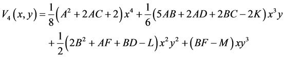
We compute the first several values below:

.

Before going any further, we note that for all degenerate foci, and also that if, then this method fails since must be one-signed. We require that the first nonzero value has an even subscript.

Definition

We say the origin of (1) is said to be a degenerate focus of odd order k if , but.

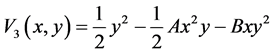
We continue by considering the equation, and solve this by choosing to avoid some computational problems that will arise later in this process. Applying the algorithm further with gives:

.

Now, setting gives the condition, so that. It then follows,

after setting, that we have. Thus, with:

.

From here, we set and get. With this extra condition,

becomes. If we make the choice, the origin will be a center,

as proved in [2] . This is not desirable, so we choose and continue:

.

Setting gives, and this condition effectively sends to 0. Com- bining this final condition with all the others gives us. Thus, in terms of Liapunov quantities, we have:

,

and, in summary, with the constraints below, the origin is a center:

.

Thus, we will have a degenerate focus at the origin of the highest order taking:

and.

2. Coexisting Weak Focus

We continue our investigation of our planar cubic system (1). We have already estab- lished criteria for this system to have three local limit cycles near the origin. Here, we wish to consider the condition that this system has a weak focus at, where, and examine whether this condition gives way to any local limit cycles near this new fixed point. Without loss of generality, we consider the case where, and extend the results accordingly.

It is easy to calculate the necessary constraints on this system for to be a fixed point, namely:

,.

Since we further require that this fixed point is a weak focus, we need that the Jacobian matrix of the system evaluated at, denoted, satisfies and. This gives us that:

, , with,.

Entering these results into the system gives us the following:

.

Next, we add in the values previously determined that give us the highest odd order degenerate focus whilst simultaneously preserving the constraints for the weak focus. Altogether, we have:

, , , , with, ,.

We then apply a transformation to take the weak focus onto the origin and write this in canonical form. This gives:

.

To analyze behavior in a neighborhood of the origin, we apply a familiar method. See Blows and Lloyd [4] for example. Recall that we may use a Liapunov function of the form:

,

where is homogeneous with degree m.

As is well known, in this case we are able to construct such that:

.

The sign of the first nonzero value determines the stability of the weak focus. If all values are zero, then we have a center. We begin our computations for the values below:

.

Setting and solving for M and L provides the possibilities, , , and. A choice of results in a symmetric center, and the two choices for L are disallowed by our earlier established constraints. We note here also that the denominator cannot be zero as a result of these same constraints. So, we take, and continue our algorithm. It then follows that:

.

If we set this to zero and solve for M, our only non-imaginary choice is, which forces a symmetric system. So, instead, we solve for N. The choice of

is disallowed, as is, and the other choice cannot occur either, as

we have established.

Hence, it follows from the equation above, paired with the constraints to preserve the third odd order degenerate focus at the origin, that this focal value cannot be zero, i.e.. So, the fixed point here is a weak focus of at least second order.

3. Results

Theorem 1

The system:

,

where, , and have a third odd order degenerate focus at the origin and a second order weak focus at. Moreover, the two foci have the same stability.

Proof. This result follows from the work carried out in the prior two sections above, and it is clear that both foci have the stability of.

□

Theorem 2

The system:

,

where, , , , , , and have three local limit cycles about the origin and one local limit cycle about.

Proof. We begin by noting if, we satisfy the hypotheses of Theorem 1 above. Now, we first perturb away from 0 such that produces a

local limit cycle about the origin, since has opposite sign to .

This perturbation leaves the other fixed point at, but the weak focus be- comes a strong focus whose stability is given by. Since, a local limit cycle has been produced about. The perturbation of away from 0 pro-

duces a second local limit cycle about the origin, since and. Lastly,

perturbing away from 0 produces a third local limit cycle about the origin since the origin becomes a strong focus whose stability is given by, which is of opposite sign to M, hence the opposite sign to.

□

Remark: Although we only considered the case for for the weak focus on the vertical axis, a similar argument can be done for any nonzero with comparable results and conclusion.

Cite this paper

Schoonover, N. and Blows, T. (2016) Co-Existence of Local Limit Cycles from Degenerate and Weak Foci in Cubic Systems. Applied Mathematics, 7, 1927-1933. http://dx.doi.org/10.4236/am.2016.716158

References

- 1. Perko, L.M. (1991) Differential Equations and Dynamical Systems. Springer Verlag, New York.
http://dx.doi.org/10.1007/978-1-4684-0392-3 - 2. Blows, T.R. (2016) Local Limit Cycles of Degenerate Foci in Cubic Systems. In: Toni, B., Ed., Mathematical Sciences with Multidisciplinary Applications, Springer, Switzerland, 21-27.
http://dx.doi.org/10.1007/978-3-319-31323-8_2 - 3. Andreev, A.F., Sadovskii, A.P. and Tsikalyuk, V.A. (2003) The Center-Focus Problem for a System with Homogeneous Nonlinearities in the case of Zero Eigenvalues. Differential Equations, 39, 155-164.
http://dx.doi.org/10.1023/A:1025192613518 - 4. Blows, T.R. and Lloyd, N.G. (1984) The Number of Limit Cycles of Certain Polynomial Differential Equations. Proceedings of the Royal Society of Edinburgh: Section A Mathematics, 98, 215-239.
http://dx.doi.org/10.1017/S030821050001341X