Applied Mathematics
Vol.4 No.11C(2013), Article ID:38688,12 pages DOI:10.4236/am.2013.411A3003
Comparison between Fourier and Wavelets Transforms in Biospeckle Signals
1Engineering Department, Federal University of Lavras, Lavras, Brazil
2Exact Science Department, Federal University of Lavras, Lavras, Brazil
3Biomathematics and Statistics Scotland, Rowett Institute of Nutrition and Health, Aberdeen, Scotland
Email: klebermariano@gmail.com, robbraga@deg.ufla.br, safadi@dex.ufla.br, g.horgan@abdn.ac.uk
Copyright © 2013 Kleber Mariano Ribeiro et al. This is an open access article distributed under the Creative Commons Attribution License, which permits unrestricted use, distribution, and reproduction in any medium, provided the original work is properly cited.
Received July 28, 2013; revised August 28, 2013; accepted September 5, 2013
Keywords: Spectral Analysis; Dynamic Speckle; Biological Activity
ABSTRACT
The dynamic speckle is a non-destructive optical technique that has been used as a tool for the characterization of the biological activity and several studies are conducted to obtain for more information about the correspondence of the observed phenomena and their expressions in the interference images. Analysis in the frequency domain has been considered as powerful alternative, and although there are works using Fourier transform in the frequency analysis of the biospeckle signals, the majority presents the wavelet transform as tool for spectral analysis. In turn, there are still doubts if the Fourier transform is not enough for the analysis of the biospeckle, which would enable the reduction of processing time since an operation is computationally simpler. In this context, the present study aims to compare the constituents’ parts of the speckle signal according to Fourier and wavelet transforms for numerical analysis. The comparative analysis based on the absolute values of the differences technique (AVD) was carried out for performance evaluation of the Fourier and wavelet transforms, in which the speckle signals were decomposed spectrally and subsequently reconstructed with the elimination of specific frequency bands. Results showed that the wavelet transform allowed more information about signals constituents of the dynamic speckle, emphasizing its use instead of the Fourier transform, which in turn was restricted the situations in which the only interest is to know the spectral content of the data.
1. Introduction
When a coherent light, such as laser, illuminates a rough surface, compared the wavelength of laser, it occurs a phenomenon of optical interference with the formation of light and dark regions, called speckle [1].
After applying the dynamic surface, there is a continuous formation of new and different speckles, and these random and dynamic interference patterns is called dynamic speckle or biospeckle, if the area concerned is biological. This technique allows extracting information about the structures movement of the illuminated material, making it an interesting tool in several knowledge areas [2].
The biospeckle has been used as a technique to measure detailed extensions of pine roots [3] or even the biological activity of roots in tissue culture [4], in assessing the water activity in maize and beans seeds [5], to studies of the relationship between chlorophyll pigments present in apples and their respective biological activity [6], and several other papers.
The biological activity expressed in the context of speckle does not present a clear definition of what phenomenon is creating, however can be understood as structural and molecular motions occurring in the material analysis [4], Doppler effect, Brownian motion, variations of the refractive index [7], among others. It is a complex signal and with causes still investigated [8], which is a challenge, and at the same time, a motivation.
In this context, the use of image processing techniques and signal analysis tools can be used in the biospeckle signal to understand better this optical phenomenon.
The interference patterns analysis can use graphical methods, which generate maps indicating the spatial variability of the biological activity, or a numerical interpretation of the temporal variation of patterns formed. An alternative of the graphical and numerical classifications is a signal analysis in the time domain or in the frequency domain [5].
The analysis of biospeckle signals in the frequency domain has been an alternative for many applications, allowing the filter and images contrast, beyond search of frequency markers of phenomena that contribute to the formation of the interference patterns in time, as described by [5]. Thereby, Fourier and wavelet transforms can be a good choice to make such analysis in the frequency domain.
Several studies have been conducted using the spectral analysis in the biospeckle signal, such as [9] that used the Fourier transform to analysis bean seeds contaminated by two kinds of fungi and managed to differentiate them using the harmonics amplitude; [10] assessed damage in apples and seed germination using wavelet transform and defined frequency markers for biological phenomena, as well as [5] who studied maize and beans, and cancer isolation and others.
Although there are many papers applying spectral analysis in the biospeckle signal, the most journals use wavelet transform and there is no works evaluating if Fourier transform, which is simpler than wavelet transform. It’s enough in the frequency analysis of the dynamic speckle. In this context, the present study aims to compare the Fourier and wavelet transform in the spectral analysis of biospeckle signal.
2. Theory
2.1. Time History of the Speckle Patterns (THSP)
The biospeckle is a nondestructive optical technique based on the analysis of the variations of the laser light scattered from material, and the biological activity presented reflects the state of the investigated object [11].
Follow a set of pixels of the images speckles in the time is a method of monitoring their time variations and consequently the biological activity of the studied object, and, in this context, [12] proposed the Time History of the Speckle Patterns (THSP).
The THSP is a two dimensional image that record a certain line or column of pixels in successive moments and arrange them vertically side by side. The x axis show information about the time evolution of the selected pixels and the y axis is the spatial distribution of the interference patterns [12].
2.2. Co-Occurrence Matrix
The co-occurrence matrix was presented by [13], and expresses the number of the transitions of each THSP pixel with respect to its immediate neighbor. Equation (1) describes mathematically the co-occurrence matrix.
 (1)
(1)
which:
 is the co-occurrence matrix,
  correspond the number of occurrences of an intensity value i, followed by an intensity value j to move through rows or columns of the time history.
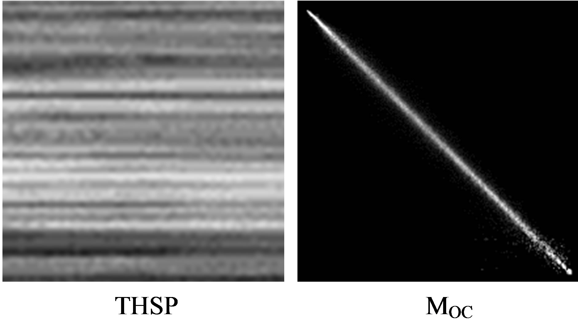
Phenomenon that show low biological activities, their time variations of the speckle patterns are slow and present a THSP horizontally in the elongated shape and the co-occurrence matrix is characterized by small changes of the pixels intensity to i and j, as illustrated in the Figure 1(a). However, materials that exhibit high biological activity shows fast intensity variations in the THSP that resemble an ordinary spatial speckle patterns and their co-occurrence matrix has nonzero elements near the main diagonal (Figure 1(b)) [14].
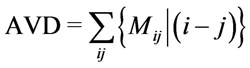
2.3. Absolute Values of the Differences (AVD)
One of the methods for analyzing of the speckle patterns is the technique of the absolute values of the differences (AVD), proposed by [15] as an alternative the inertial moment technique.
The AVD method is a statistics moment of first order which it is applied on the co-occurrence matrix and generates a number [11] which allow quantify the biological activity of the studied material. Equation (2) presents mathematically the AVD technique
 (a)
(a)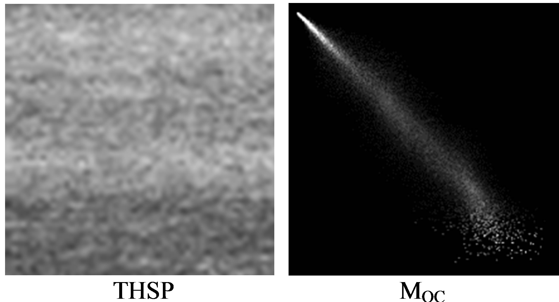 (b)
(b)
Figure 1. Time history of the speckle patterns and their respective co-occurrence matrix. Materials with low (a) and high (b) biological activity.
 (2)
(2)
which:
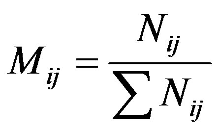
AVD is a dimensionless value, i and j are coordinates of the row and column respectively, and Mij is called of modified co-occurrence matrix and that is presented in Equation (3).
 (3)
(3)
According [15], the inertial moment showed to be more sensitive than AVD on analyzing processes that involve high biological activities, although when this variation is not so intense, this method is less efficient.
2.4. Fourier Transform
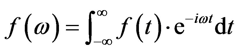
Information of the biospeckle data in the frequency domain has been an alternative to the interpretation of the interference patterns [5], with the possibility of improve the visualization of some phenomena of the studied material and to know their spectral signatures. In this context, the Fourier transform is one of the tools that can be used to spectral analysis of the biospeckle.
Fourier transform can be understood as the mathematical technique that transforms a signal from the time domain to the frequency domain, and it is formed by a set 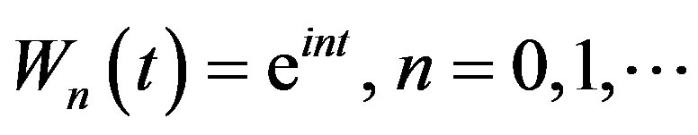 of orthogonal functions, of period 2π [16]. Equation (4) described mathematically the Fourier transform.
 (4)
(4)
which:
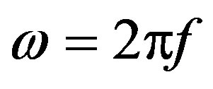
 = amplitude of each component ω of the signal.
There is also the inverse Fourier transform, which is used to transform the signal from frequency domain to time domain with the reconstruction of the original function. Equation (5) presents the mathematical expression of the inverse Fourier transform.
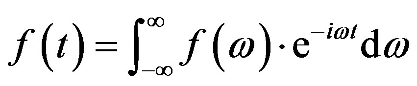 (5)
(5)
The Fourier transform indicates the spectral information of the signal without providing the instant which these components happen, and in situations that to know when the frequencies occur are interesting precludes the use of Fourier transforms, unless if the series is stationary [17]. In this context, the wavelet transform is an alternative that provides the instant the frequency components occur.
2.5. Wavelets Transform
The wavelets are simply waves of duration adjusted with energy concentrated in variables intervals [18], which makes it a great useful method for time series analysis, that exhibit characteristics that can change in the time and in frequency.
The continuous wavelet transform is defined as the convolution of  with a scaled and translated version of
  [19], called wavelet mother. Equation (6) describes mathematically the continuous wavelet transform.
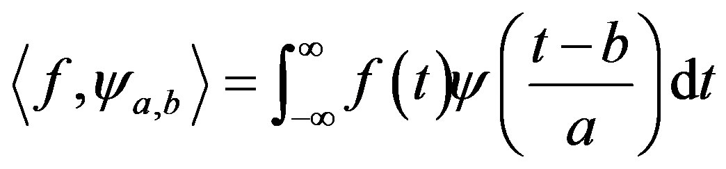 (6)
(6)
which:
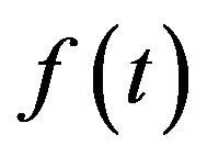 is the studied signal a scale parameter b translation value
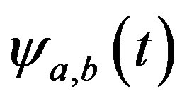 is the mother function of wavelets
 is the spectrum wavelets.
The scale is related to the frequency, in which high scales correspond to low frequencies and low scales correspond to high frequencies, whereas the translation is the displacement of the mother function about the studied signal [20].
The return of the signal from frequency domain to time domain, inverse wavelets transform, allows observe the behavior of the signal in specifics frequencies bands and also the reconstruction of the original function . According [19], the inverse wavelet transform can be realized by the sum of real part of wavelet spectrum on all scales (Equation (7)).
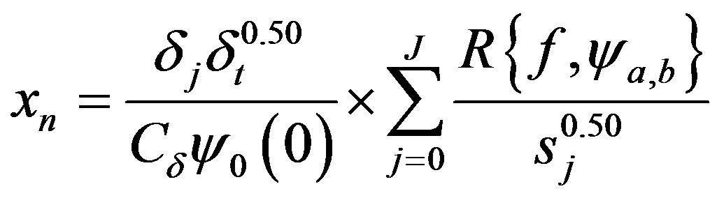 (7)
(7)
which:
 is a factor that convert the wavelets transform in energy density,
 ;
; ;
; ;
;  are specific constants of the base function used.
One of the major difficulties in wavelet analysis is the identification of the scales set used in the wavelet transform. Orthogonal wavelet, there is a limit and a discrete set of scales, as given by [21], however, for analysis of non-orthogonal wavelet, can use an arbitrary scales set to build a more complete signal [19].
In this context, [19] suggested Equations (8) and (9) to calculate the scales interval to be used in the wavelet transform, in which sj is the lowest and J is the highest scale.
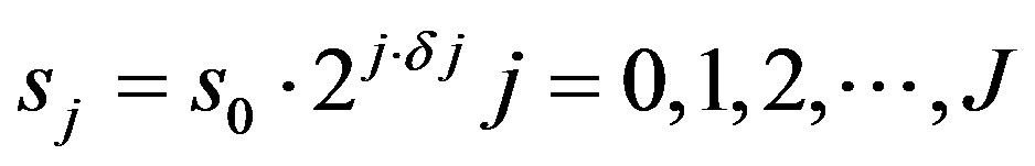 (8)
(8)
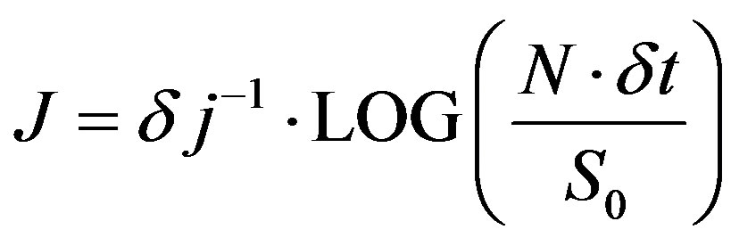 (9)
(9)
The s0 should be chosen so that the Fourier period is , and to the Morlet wavelet the largest value that can adjust the scale is
  of 0.5. For other wavelet functions can be used a larger value.
2.6. Sampling Theorem
The sampling theorem describes the relationship between sampling frequency of a signal and the frequency maximum of the reconstructed signal. Below is transcript the sampling theorem as presented by [22].
“Theorem 1: If a function  contains no frequencies higher than W cps, it is completely determined by giving its ordinates at a series of points spaced 1/2 seconds W apart”.
According to the theorem, the number of samples per unit time of a signal is called rate or frequency sampling (W), and half the sampling frequency corresponds to the frequency maximum of the signal which can be reproduced in full without aliasing error.
The sampling theorem is used in this work to define the highest frequently during the decomposition of signals.
3. Materials and Methods
It was conducted a comparison between Fourier and wavelet transforms using the time history of speckle patterns (THSP) relative to a paint drying process and presented by [23].
The database was formed by 8 THSP’s collected each 20 minutes during the paint drying using the back-scattering experimental setup. Each time history was made by a set of 128 images, resolution of 512 by 640 pixels, whose time acquisition between images was of 0.08 seconds (sampling frequency of 12.5 Hz).
The lines of the THSPs were concatenated creating a new signal that was decomposed into frequency spectra using Fourier and wavelet transforms with application posterior of the inverse transform. Some frequency bands were eliminated before the reconstruction of the signal in order to analyze the results of the speckle signal using a numerical method to measure the speckle activity. The selective filtering was conducted as well in order to create some frequency markers linked to the physical phenomena under monitoring.
According the sampling theorem the highest frequency that can be seen in the reconstruction process is 6.25 Hz, and using Equations (8) and (9) were calculated the number of frequency bands used in the transform. In addition, in the continuous wavelet transform was used mother function of Morlet, a damped complex exponential with a set of oscillation parameter that preserves an approximate relationship between the scale of the wavelet analysis and the frequency in a Fourier analysis, as described by [24].
The signal resulting of the inverse transform was converted to THSP format again and numerically analyzed using the technique of the absolute values of the differences (AVD) [15], and their values compared to the gravimetrical measurement.
Figure 2 illustrated all the methodology used.
4. Results and Discussion
Figure 3 presents the absolute value of the differences for the THSP’s of the paint drying process with decomposition and reconstruction of some frequency bands using Fourier transform.
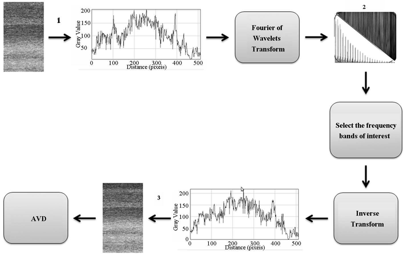
Figure 2. Methodology used to the data analysis, in which 1 represents the concatenation, 2 is the Fourier or wavelets spectrum and 3 corresponds to the inverse process of the concatenation.
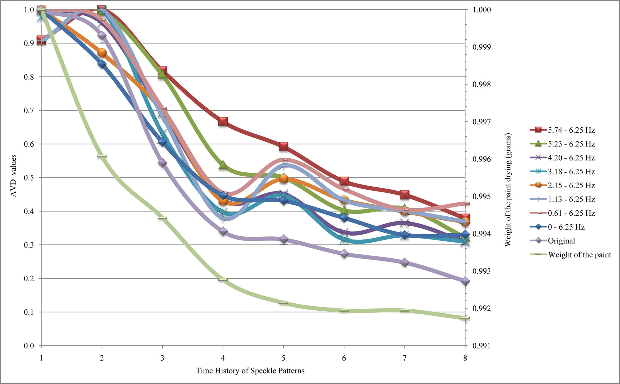
Figure 3. AVD values of the THSP’s of the paint drying using Fourier transform for spectral analysis.
The data reconstructed in the frequency band from 0 to 6.25 Hz (Figure 3), here called of total reconstruction, correspond to highest reconstruction possible in accordance with the sampling theorem, and the original data are the AVD values of the time history of the paint drying without filtering.
The dynamic speckle signals reconstructed in frequencies bands 5.74 - 6.25 and 5.23 - 6.25 Hz presented gradual reduction of AVD values along of the paint drying process, closer to the behavior of the original data, total reconstruction and to the weight of the paint drying. However, the addition of low frequencies components in the reconstruction process resulted in the oscillation of the AVD values in the fifth time history, as observed in Figure 3. We attribute those oscillations to the influence of the atmospheric conditions that occur in experiment of paint drying as the realized by [23], which did not interfered in the first moments since the paint volatility was higher and thus undermined the presence of the modulation of the signal in low frequencies linked to the atmospheric conditions such as temperature and humidity, and Figure 4 illustrates these information’s.
Figure 4 presents that the signals reconstructed with components of low frequencies (associated the temperature and humidity variables) are mixed with the data reconstructed using components of high frequencies (linked the volatility) in the first moments, and which along the paint drying process, the paint volatility stabilize and make possible to observe the high oscillations of the data reconstructed using low frequencies component.
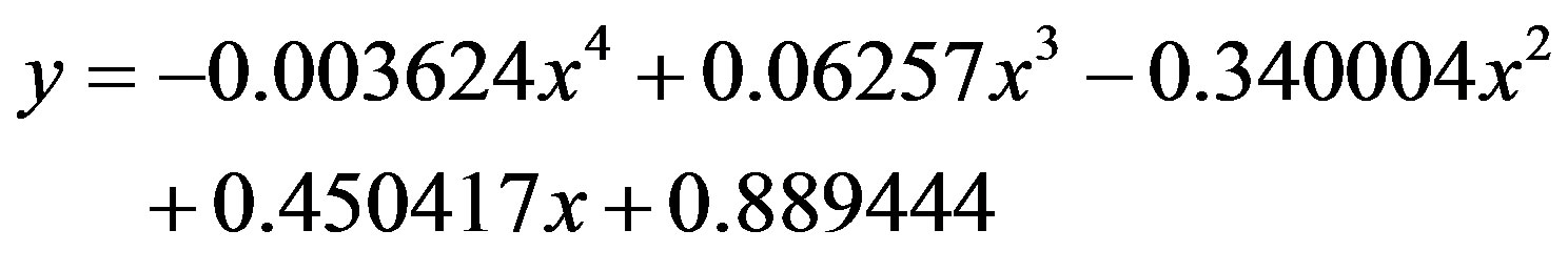
In order to clarify the spectral information found in the fifth THSP, a mathematical model was adjusted in the AVD values of the original data, using the least squares method, to describe the process of paint drying. Equation (10) presents the mathematical model adjusted and Figure 5 illustrates the regression curve.
 (10)
(10)
which:
x is the TSHP numbery is the normalized AVD value.
The mathematical model adjusted showed a correlation index of 0.98 and mean square error of 0.0048 with respect to the original.
The first derivative of the adjusted model,
 when equaled to zero, showed that the region the fifth THSP is a minimum local, and this means that the AVD values reaches a minimum value and then initiates an oscillations related to the variations of the temperature and humidity. These results are similar to the behavior of the paint weight at time presented by [23] (Figure 5), in which is possible to observe a stabilization of the weight
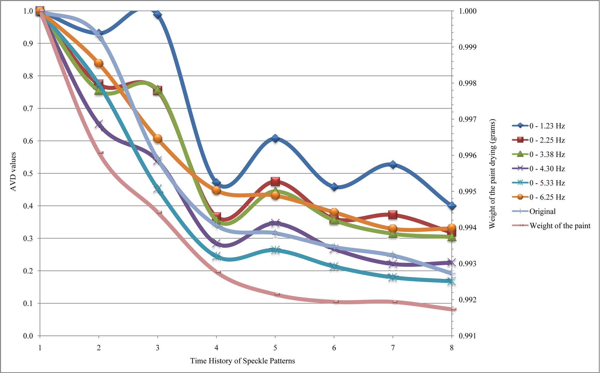
Figure 4. AVD values of the time history of the paint drying reconstructed with some frequencies band using Fourier transform.
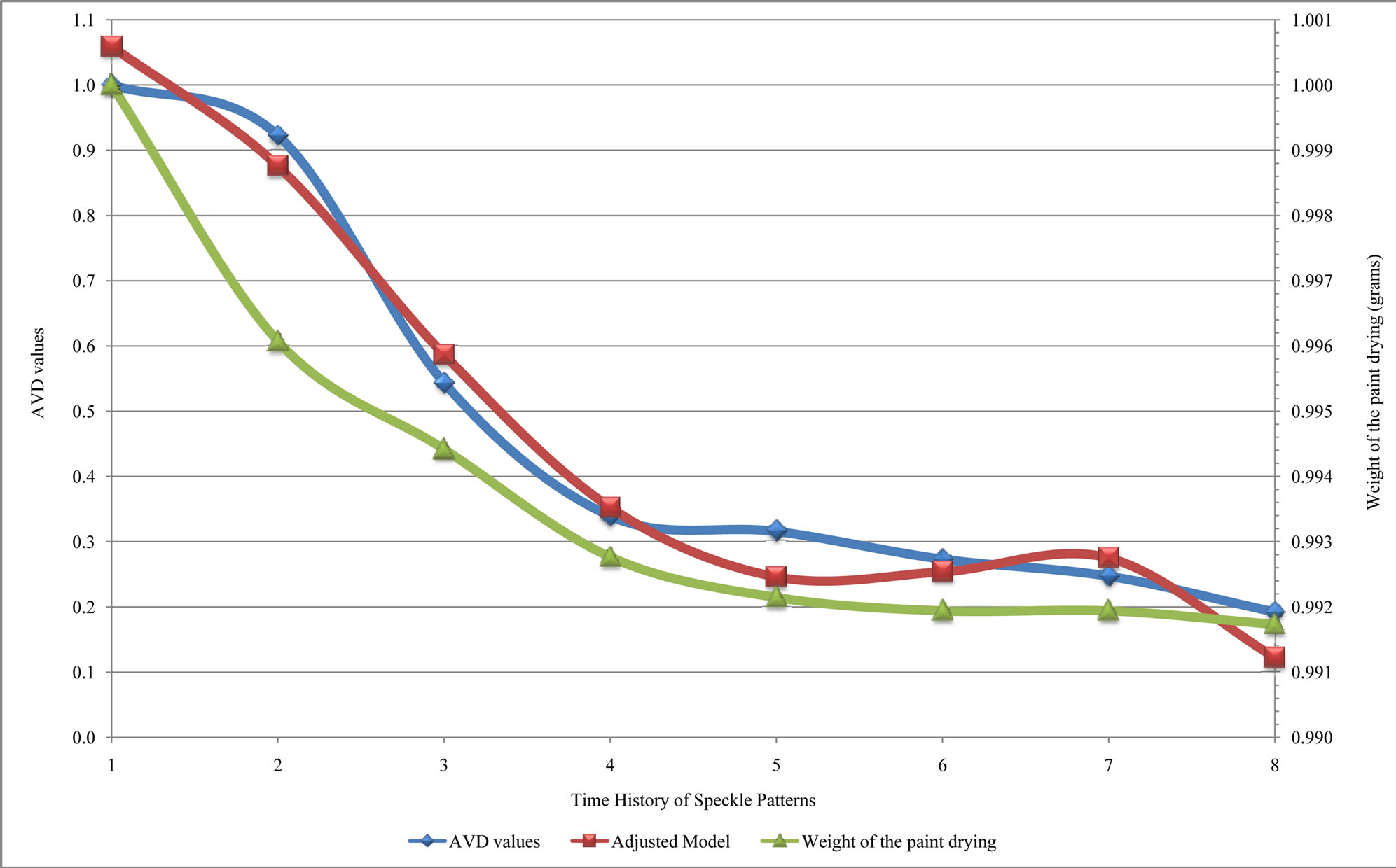
Figure 5. Regression adjusted to describe the paint drying process.
values after the fifth data acquisition, and leads us to assume that the drying time of this paint is one hour and twenty minutes, approximately. In this context, the dynamic speckle analyzed by Fourier transform allowed to observe this transition occurred in paint drying structure.
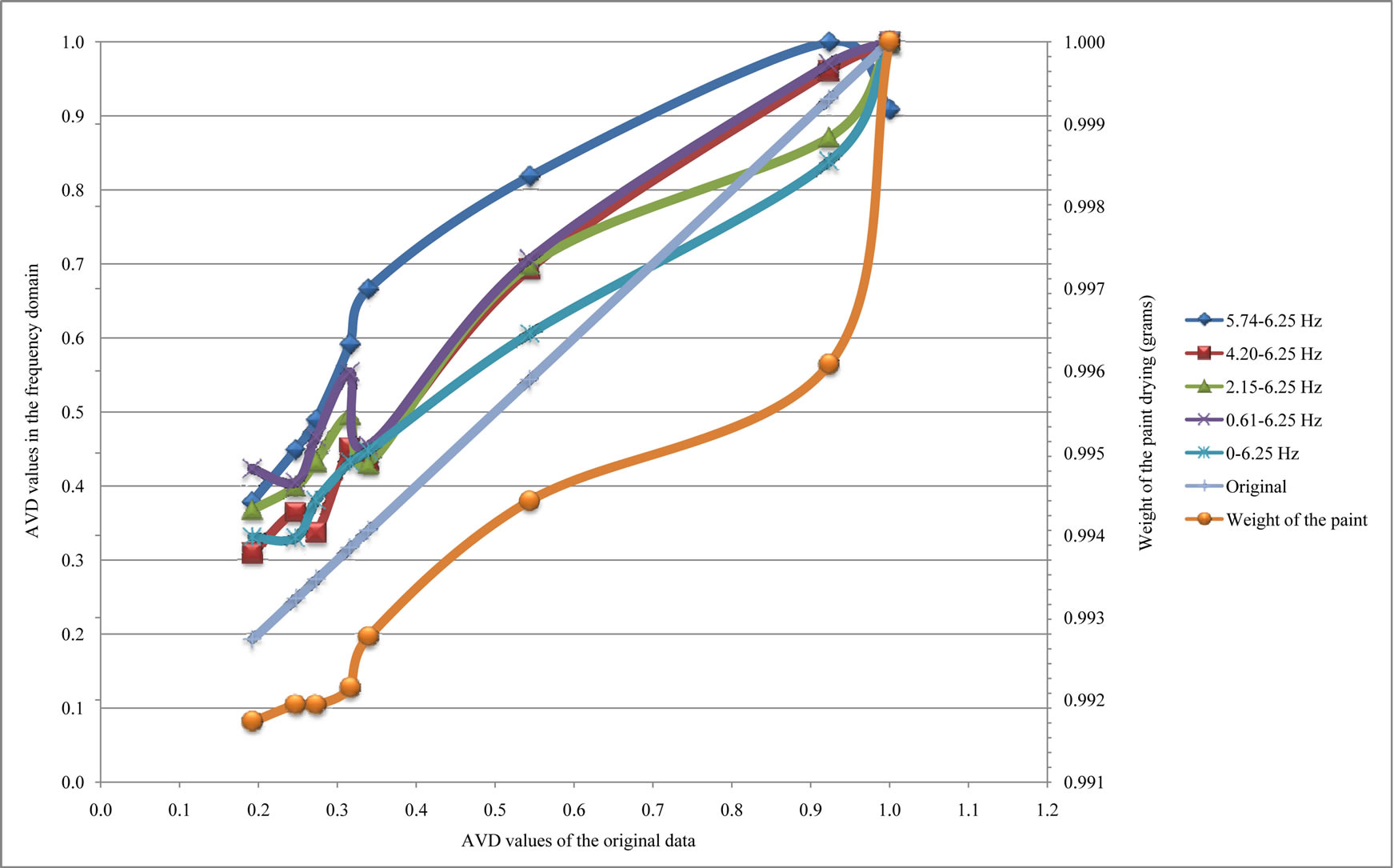
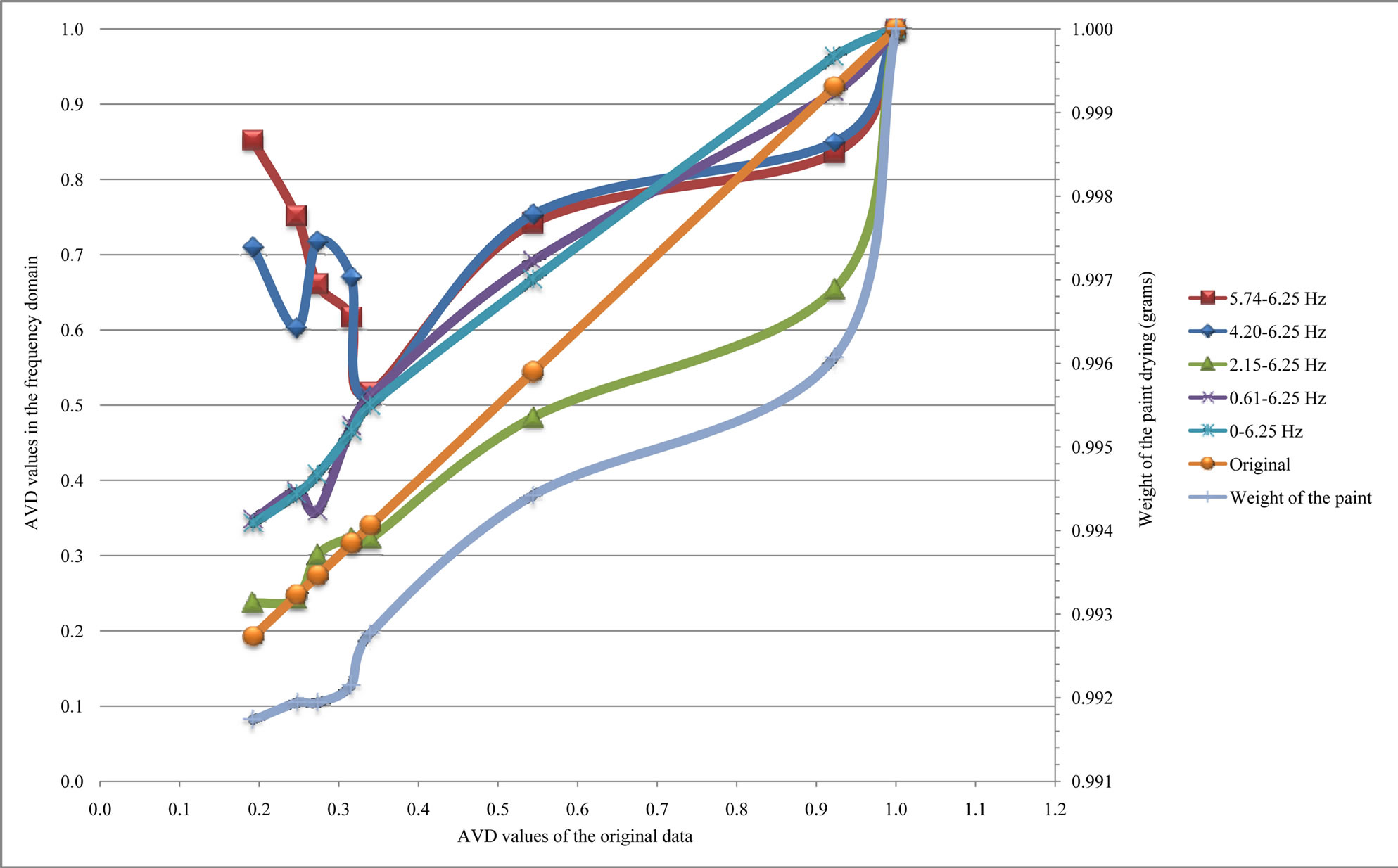
In addition, the distance between the original signals and reconstructed signals were evaluated and the results are illustrated in Figure 6.
 (a)
(a)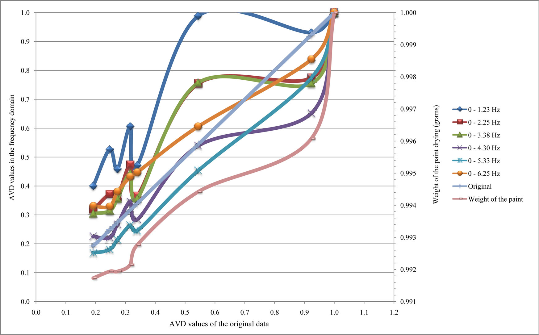 (b)
(b)
Figure 6. Signals reconstructed in specific frequency bands by inverse Fourier transform and the original signal. (a) Addition of components of low frequencies in the signals reconstruction and (b) increase high frequencies components in the inverse transform.
The largest distances were observed in the signals reconstructed using few spectral components and these distances between original signals and reconstructed signals were reducing to use a larger number of components in the inverse Fourier transform, as waited.
In addition, the correlation index between the original signal and the signals reconstructed in the frequencies bands of 5.74 - 6.25, 5.23 - 6.25 and 4.20 - 6.25 Hz were of 0.86, 0.94 and 0.98, respectively. The high correlation of 0.86 using just a small portion of the frequency band can be explained by compact support of the Fourier basis functions in the frequency domain, which allows using in data compression with minimum loss of information, as discussed by [16].
The speckle signals is not stationary [25], unviable to use the Fourier transform. Thus, frequency analysis using the Fourier transform is restricted to situations in which are interesting to know the spectral information of the data.
Otherwise, the spectral analysis using the wavelet transform presented different behavior in the high frequencies and the signal reconstructed using more components of low frequencies made the results closer to the original signal, as illustrated in Figure 7.
The total reconstruction of the biospeckle signal, in the frequency band from 0 to 6.25 Hz, showed behavior similar to the original data and to the weight of paint drying, with the gradual reduction of the AVD values in the time.
Furthermore, removing the low frequency components in the reconstruction process resulted in oscillations in the AVD values, in special, in the signals reconstructed within the frequency range from 4.20 to 6.25 Hz, which the AVD values decreasing until the fourth time history and subsequently increasing.
In this context, the high AVD values of the last time history in the frequency bands 4.20 - 6.25 Hz are attributed the random oscillations and noise presents in the biospeckle signal, without significant information’s about the paint volatility, since that the energy of the time history in the high frequencies showed was reducing along of the paint drying and presented low values after of the fourth THSP, as illustrated graphically in Figure 8.
The energy of the THSP’s (Figure 8) is represented in pseudo-colors, the ordinate axis correspond the scales and in the abscissas axis is the time. The light pseudocolors indicate high energy while dark shades are associated the low energy, and the scales are inversely proportional to the frequencies, which the low scales are attached with high frequencies and high scales with the low frequencies.
It is possible to observe in Figure 8 that the pseudocolors in the high frequencies (low scales) are darkening in the time, which means reduce of the energy in high

Figure 7. AVD values of the time history of speckle patterns of paint drying using wavelet transform for spectral analysis.
frequency bands along of the paint drying and which does not justify the high AVD values in the last time histories.
The reconstruction of the signals using components of low frequencies was also analyzed, and Figure 9 shows the results.
In the first moments we see that the signals reconstructed using components of low frequency and of high frequency mixed, instant in which the paint volatility was intense. Over time, the phenomena linked to the high frequencies stabilized, allow to observe the oscillations of the signals reconstructed with components of low fre-
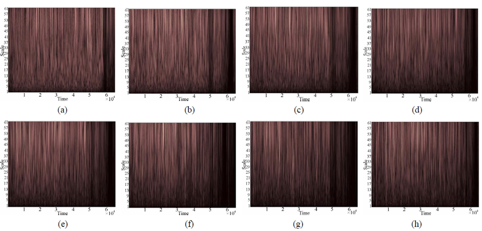
Figure 8. Energy of the 8 THSP’s for different frequencies.
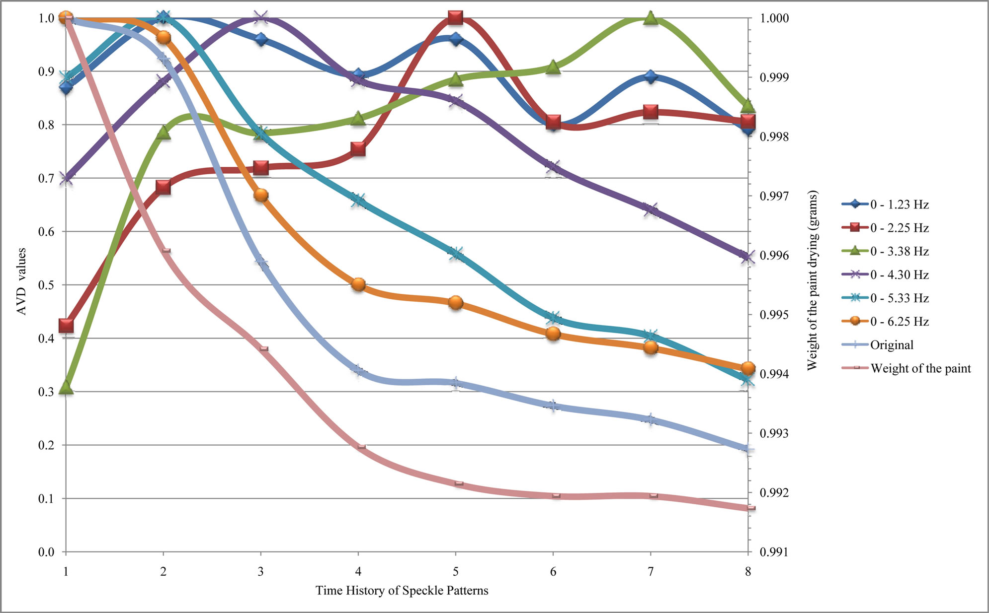
Figure 9. Absolute value of the difference of the THSP’s of the paint drying using wavelet transform for spectral analysis.
 (a)
(a)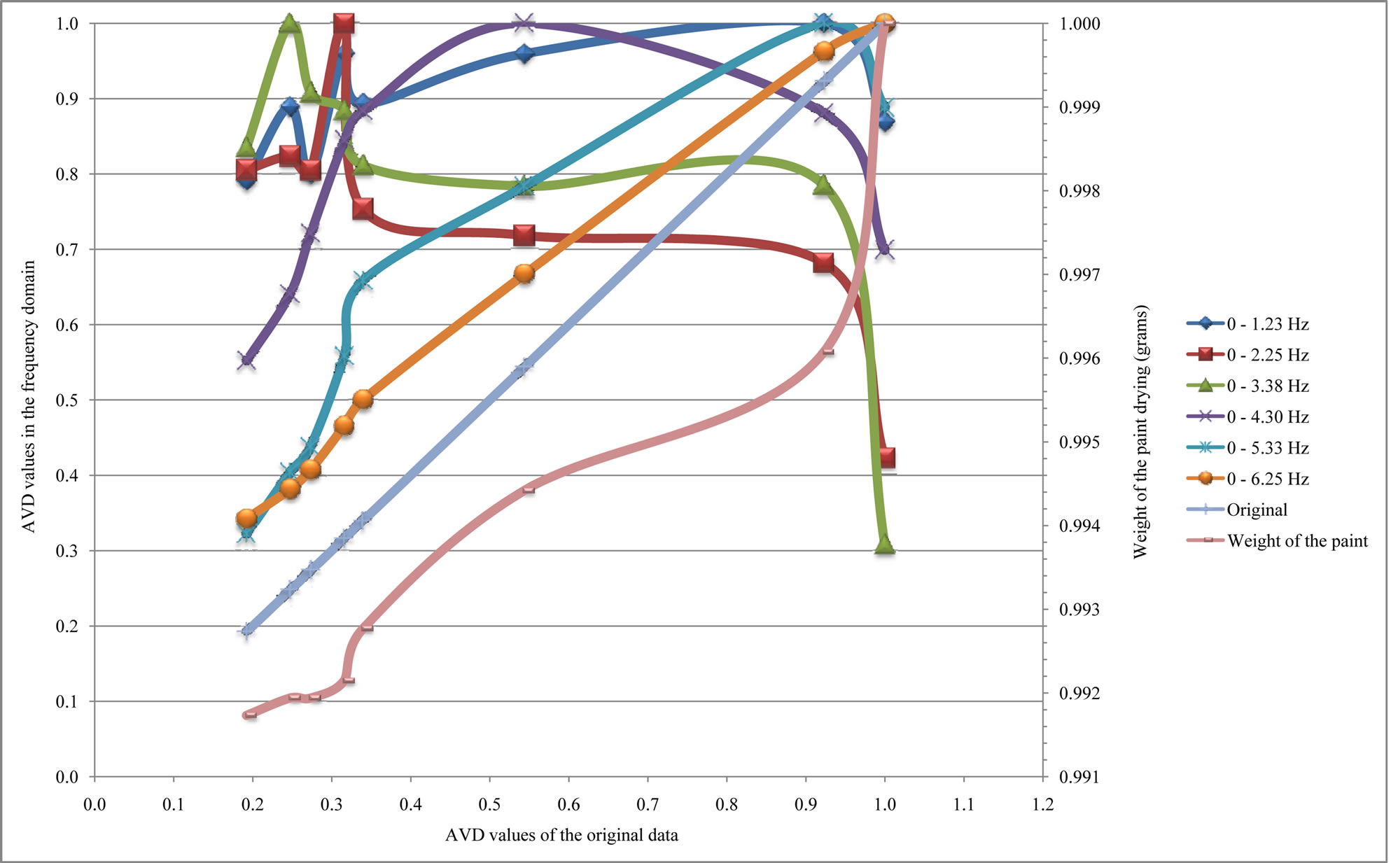 (b)
(b)
Figure 10. Signals reconstructed using wavelet transform and the original signal. (a) Addition of components of low frequencies in the inverse wavelet transform and (b) increase high frequencies components in the signal reconstruction.
quency, as the humidity and the temperature.
The reconstruction of the signals showed correlation index higher than 0.90 with the original signal when used a wide frequency band, the opposite showed when we used the Fourier transform. Figure 10 presents the signals reconstructed using wavelet transform against the original signal, and allow observation the distance between the curves when we added components of high and low frequencies in the reconstruction of the signals.
Signals reconstructed in frequency bands of 5.23 - 6.25, 4.20 - 6.25 and 3.18 - 6.25 Hz presented correlation index of 0.30, 0.69 and 0.92, respectively. The Morlet function does not have compact support, which explains the need for a large number of spectral components for great approximation of the original signal. Furthermore, the addition of components of low frequencies (Figure 10(a)) and of high frequencies (Figure 10(b)) in the signal reconstruction made the reconstructed data closer to the original signal.
In this context, the wavelet transform details spectral information’s in time, which does not occur in the Fourier transform, and that in the analysis of the biospeckle signals provides further information of the studied process and facilitates to understand the signals that create this complex phenomenon of optical interference, being the adequate tool for studies in the frequency domain.
5. Conclusion
The Fourier transform allowed data analysis with compact support, while the wavelets provided definition of frequency markers and information is not presented in the Fourier analysis about the participants of the dynamic speckle signal and being the tool that most adequate for frequency analysis.
6. Acknowledgements
This work was partially financed by CNPq, Fapemig, Capes, Finep in Brazil, and partly supported by the Scottish Government Rural and Environment Science and Analytical Services division.
REFERENCES
- Y. Zhao, J. Wang, X. Wu, F. W. Williams and R. J. Schmidt, “Point-Wise and Whole-Field Laser Speckle Intensity Fluctuation Measurements Applied to Botanical Specimens,” Optics and Lasers in Engineering, Vol. 28, No. 6, 1997, pp. 443-456. http://dx.doi.org/10.1016/S0143-8166(97)00056-0
- H. J. Rabal and R. A. Braga, “Dynamic Laser Speckle and Applications,” CRC Press, New York, 2008.
- A. P. Rathnayake, H. Kadono, S. Toyooka and M. Miwa, “A Novel Optical Interference Technique to Measure Minute Root Elongations of Japanese Red Pine (Pinusdensiflora Seibold & Zucc.) Seedlings Infected with Ectomycorrhizal Fungi,” Environmental and Experimental Botany, Vol. 64, No. 3, 2008, pp. 314-321. http://dx.doi.org/10.1016/j.envexpbot.2008.02.007
- R. A. Braga, L. Dupuy, M. Pasqual and R. R. Cardoso, “Live Biospeckle Laser Imaging of Root Tissue,” European Biophysics, Vol. 38, No. 5, 2009, pp. 679-686. http://dx.doi.org/10.1007/s00249-009-0426-0
- R. R. Cardoso, A. G. Costa, C. M. B. Nobre and R. A. Braga, “Frequency Signature of Water Activity by Biospeckle Laser,” Optics Communications, Vol. 284, No. 8, 2011, pp. 2131-2136. http://dx.doi.org/10.1016/j.optcom.2011.01.003
- A. Zdunek and W. B. Herppich, “Relation of Biospeckle Activity with Chlorophyll Content in Apples,” Postharvest Biology Technology, Vol. 64, No. 1, 2012, pp. 58-63. http://dx.doi.org/10.1016/j.postharvbio.2011.09.007
- I. Passoni, A. Dai Pra, H. J. Rabal, M. Trivi and R. Arizaga, “Dynamic Speckle Processing Using Wavelets Based Entropy,” Optics Communications, Vol. 246, No. 1-3, 2005, pp. 219-228. http://dx.doi.org/10.1016/j.optcom.2004.10.054
- R. M. Costa, T. Sáfadi, G. F. Rabelo and R. A. Braga, “Té- cnicas Estatísticas Aplicadas em Imagens do Speckle Dinâmico,” Revista Brasileira de Biometria, Vol. 28, No. 2, 2010, pp. 27-39.
- G. F. Rabelo, A. M. Enes, R. A. Braga and I. M. Dal Fabbro, “Frequency Response of Biospeckle Laser Images of Bean Seeds Contaminated by Fungi,” Biosystems Engineering, Vol. 110, No. 3, 2011, pp. 297-301. http://dx.doi.org/10.1016/j.biosystemseng.2011.09.002
- G. H. Sendra, R. Arizaga, H. Rabal and M. Trivi, “Decomposition of Biospeckle Images in Temporary Spectral Bands,” Optics Letters, Vol. 30, No. 13, 2005, pp. 1641- 1643. http://dx.doi.org/10.1364/OL.30.001641
- M. D. Z. Ansari and A. K. Nirala, “Assessment of the BioActivity Using the Methods of Inertia Moment and Absolute Value of the Differences,” Optiks—International Journal for Light and Electron Optics, Vol. 124, No. 15, 2013, pp. 2180-2186.
- G. Oulamara, J. Tribillon and J. Duvernoy, “Biological Activity Measurements on Botanical Specimen Surfaces Using a Temporal Decorrelation Effect of Laser Speckle,” Journal of Moderns Optics, Vol. 36, No. 2, 1989, pp. 136-179. http://dx.doi.org/10.1080/09500348914550221
- R. Arizaga, M. Trivi and H. Rabal, “Speckle Time Evolution Characterization by the Co-Occurrence Matrix Analysis,” Optics and Laser Technology, Vol. 31, No. 2, 1999, pp. 163-169. http://dx.doi.org/10.1016/S0030-3992(99)00033-X
- R. A. Braga, I. M. Dal Fabbro, F. M. Borém, G. F. Rabelo, R. Arizaga, H. Rabal and M. Trivi, “Assessment of Seed Viability by Laser Speckle Techniques,” Biosystems Engineering, Vol. 86, No. 3, 2003, pp. 287-294. http://dx.doi.org/10.1016/j.biosystemseng.2003.08.005
- R. A. Braga, C. M. B. Nobre, A. G. Costa, T. Sáfadi and F. M. Costa, “Evaluation of Activity through Dynamic Laser Speckle Using the Absolute Value of the Differences,” Optics Communications, Vol. 284, No. 2, 2011, pp. 646- 650. http://dx.doi.org/10.1016/j.optcom.2010.09.064
- P. A. Morettin, “Ondas e Ondeletas,” EDUSP, São Paulo, 1999.
- M. Sifuzzaman, M. R. Islam and M. Z. Ali, “Application of Wavelet Transform and Its Advantages Compared to Fourier Transform,” Journal of Physical Sciences, Vol. 13, No. 1, 2009, pp. 121-134.
- A. Graps, “An Introduction to Wavelets,” Computation Science and Engineering, IEEE, Vol. 2, No. 2, 1995, pp. 50-61. http://dx.doi.org/10.1109/99.388960
- C. Torrence and G. P. Compo, “A Practical Guide to Wavelet Analysis,” Bulletin of the American Meteorological Society, Vol. 79, No. 1, 1998, pp. 61-78. http://dx.doi.org/10.1175/1520-0477(1998)079<0061:APGTWA>2.0.CO;2
- H. R. Karimi, W. Pawlus and K. G. Robbersmyr, “Signal Reconstruction, Modeling and Simulation of a Vehicle Full-Scale Crash Test Based Morlet Wavelets,” Neurocomputing, Vol. 93, No. 15, 2012, pp. 88-99. http://dx.doi.org/10.1016/j.neucom.2012.04.010
- M. Farge, “Wavelet Transforms and Their Applications to Turbulence,” Annual Review of Fluid Mechanics, Vol. 24, No. 1, 1992, pp. 395-457. http://dx.doi.org/10.1146/annurev.fl.24.010192.002143
- C. E. Shannon, “Communication in the Presence of Noise,” Proceedings of the IRE, Vol. 37, No. 1, 1949, pp. 10-21. http://dx.doi.org/10.1109/JRPROC.1949.232969
- M. M. Silva, J. R. A. Nozela, M. J. Chaves, R. A. Braga and H. Rabal, “Optical Mouse Acting as Biospeckle Sensor,” Optics Communications, Vol. 284, No. 7, 2011, pp. 1798-1802. http://dx.doi.org/10.1016/j.optcom.2010.12.037
- L. Polansky, G. Wittemyer, P. C. Cross, C. J. Tambling and W. M. Getz, “From Moonlight to Movement and Synchronized Randomness: Fourier and Wavelet Analyses of Animal Location Time Series Data,” Ecology, Vol. 91, No. 5, 2010, pp. 1506-1518. http://dx.doi.org/10.1890/08-2159.1
- H. Sendra, S. Murialdo and L. Passoni, “Dynamic Laser Speckle to Detect Motile Bacterial Response of Pseudomonas Aeruginosa,” Journal of Physics: Conference Series, Vol. 90, No. 1, 2007, pp. 1-6.