Applied Mathematics
Vol. 4 No. 8A (2013) , Article ID: 35076 , 5 pages DOI:10.4236/am.2013.48A003
SEIR Model and Simulation for Vector Borne Diseases
Department of Mathematics, Gujarat University, Ahmedabad, India
Email: nitahshah@gmail.com, guptajyoti.gu@gmail.com
Copyright © 2013 Nita H. Shah, Jyoti Gupta. This is an open access article distributed under the Creative Commons Attribution License, which permits unrestricted use, distribution, and reproduction in any medium, provided the original work is properly cited.
Received April 17, 2013; revised May 17, 2013; accepted May 24, 2013
Keywords: SEIR-Model; Vector Borne Disease; Malaria; Simulation
ABSTRACT
An epidemic model is a simplified means of describing the transmission of infectious diseases through individuals. The modeling of infectious diseases is a tool which has been used to study the mechanisms by which diseases spread, to predict the future course of an outbreak and to evaluate strategies to control an epidemic. Epidemic models are of many types. Here, SEIR model is discussed. We first discuss the basics of SEIR model. Then it is applied for vector borne diseases. Steady state conditions are derived. A threshold parameter R0 is defined and is shown that the disease will spread only if its value exceeds 1. We have applied the basic model to one specific diseases-malaria and did the sensitivity analysis too using the data for India. We found sensitivity analysis very important as it told us the most sensitive parameter to be taken care of. This makes the work more of practical use. Numerical simulation is done for vector and host which shows the population dynamics in different compartments.
1. Introduction
Mathematical epidemiology seems to have grown exponentially starting in the middle of 20th century. A huge variety of models have been formulated, mathematically analyzed and applied to infectious diseases.
Nedelman [1] presented the review of the work done in the field of malaria modeling. Aron [2] modeled the immunity to this disease. Ngwa and Shu [3] designed and analyzed the model for malaria when it was in endemic situation. Sheikh [4] analyzed an SEIR model with limited resources for treatment. Method for analyzing a general compartmental model was given by Drissche and Watmough [5]. Jones [6] has given the details on basic reproduction number R0. Simulation is carried out in MATLAB [7]. Basics of epidemic modeling are explained in [8].
The idea behind compartmental models is to divide the entire population into sets of different classes according to its epidemiological status. Epidemic models are of many types depending upon the number of compartments considered in it.
In this paper, Section 2 gives model formulation and its analysis. A threshold parameter R0 is also discussed in this section. Next, in Section 3, we apply this model to vector borne diseases. Sensitivity analysis is done using values of different parameters in Indian context. These values are given in Table 1. The results of sensitivity analysis are given in Table 2. Simulation is done using MATLAB and is given in Section 5. Here, Figure 1 shows the trends of human population in different compartments and Figure 2 shows the same for mosquito population.
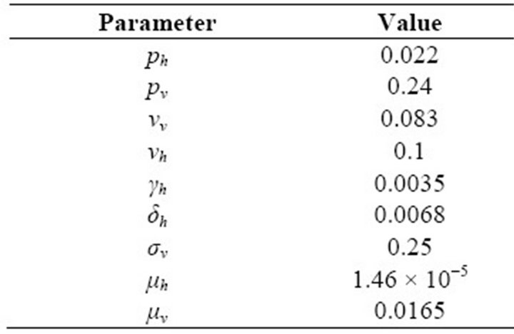
Table 1. Values of Parameters.
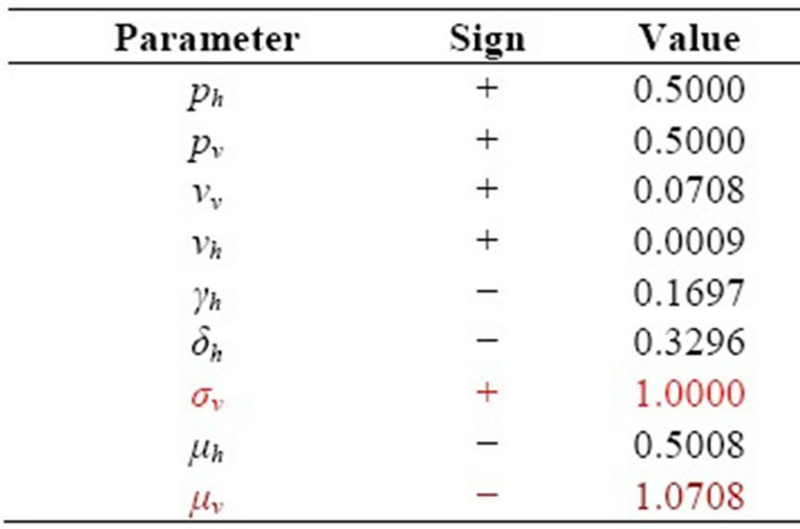
Table 2. Sensitivity Indices of R0 to the parameters for the malaria model.
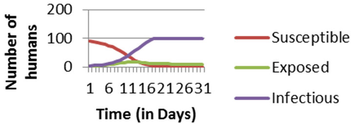
Figure 1. Numerical Simulation of Human Population considering entire population to be susceptible at the initial stage.
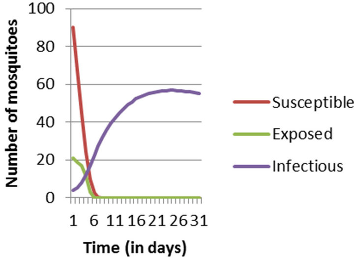
Figure 2. Numerical Simulation of Mosquito Population considering entire population to be susceptible at the initial stage.
2. Mathematical Model
Here, we discuss SEIR epidemic model (Plate 1) that have compartments Susceptible, Exposed, Infectious and Recovered.
We prefer this compartmental model over others as it takes care of latent period i.e. exposed class which is left in SIR or SIS etc. Also it does not make the things too complicated as in the models with more compartments.
2.1. Assumptions
Let us call S, E, I and R the number of the members of each class. We now make assumptions regarding the transmission and incubation periods:
1) The number of infected people increases at a rate proportional to both the number of infectious and the number of susceptible i.e. βSI with β > 0. So, the number
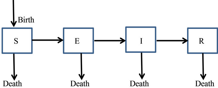
Plate 1. The general transfer diagram for SEIR epidemic model.
of susceptible will decrease at the same rate. Here, β is called the effective infection rate.
2) Individuals from exposed class will move to infectious class with a rate ν (progression rate).
3) The rate of removal of infectious to recovered compartment is proportional to the number of infectious only i.e. γI with γ > 0. Here, γ is called removal rate.
4) A person can die at any stage by natural causes. Therefore μ is taken as natural death rate and δ as disease induced death rate.
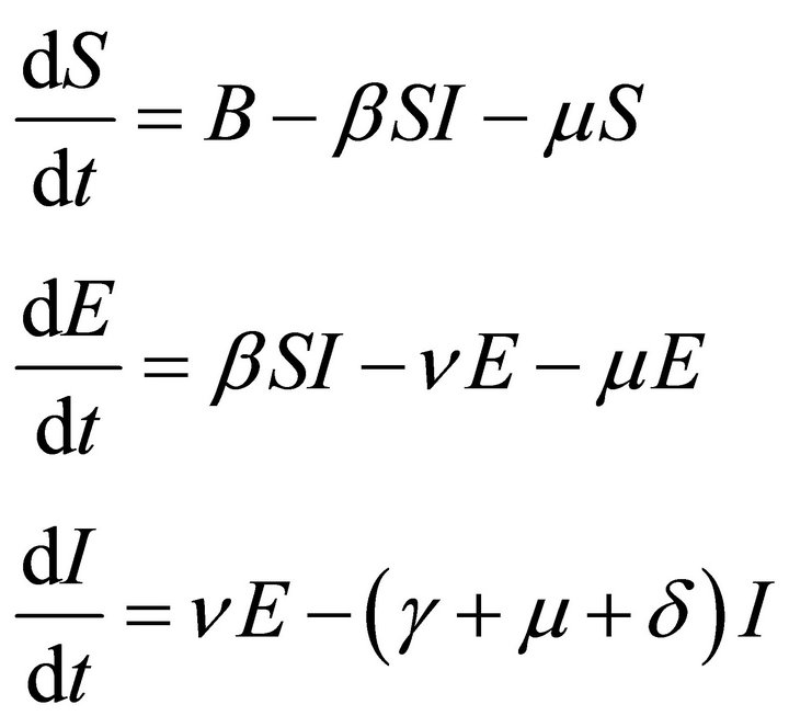
2.2. Model
The model takes the form
 (1)
(1)
with S > 0, E ≥ 0, I > 0, R ≥ 0.
Here, B is new recruitment by birth etc.
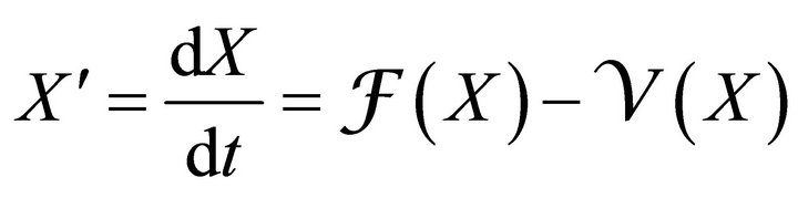
Since an epidemic occurs in a short time period, we ignore loss of temporary immunity. Therefore, we have no transfer from the recovered compartment back to the susceptible compartment. Thus R does not appear in any of the first three equations. So, we will analyse the first three equations forming new reduced system as
 (2)
(2)
Adding above three equations of system (2), we have
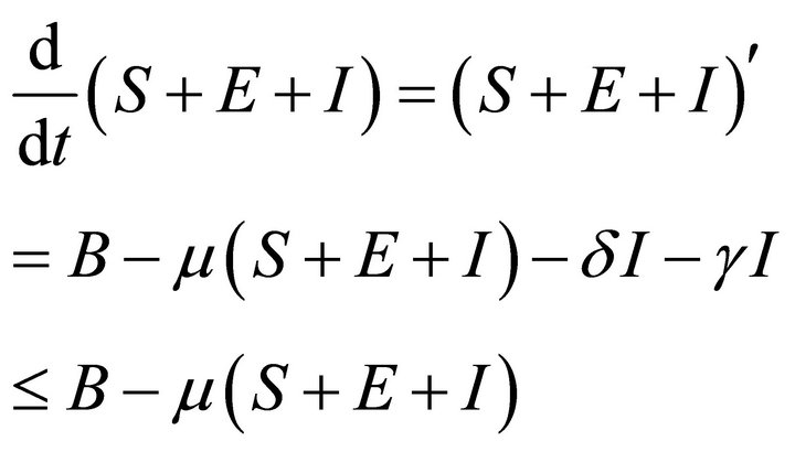
Then
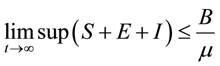
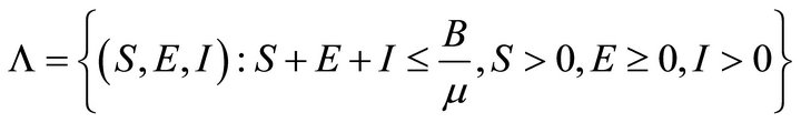
So, the feasible region for (2) is
Now the basic reproduction number R0 will be found by using the next generation matrix found in Driessche and Watmough (2002).
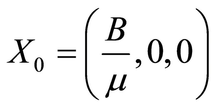
It is easy to see that (2) always has a disease free equilibrium.
Therefore, here, I has to be less than its initial value I0 (say). Let .
.
Therefore
 (3)
(3)
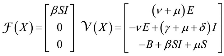
where  gives the rate of appearance of new infections in a compartment and
  gives the transfer of individuals. And
 (4)
(4)
Since,  is a disease free equilibrium of (3), therefore the derivatives
  and
and 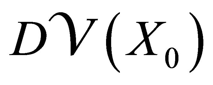 are partitioned as
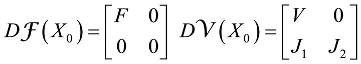
where F and V are 2 × 2 matrices defined as
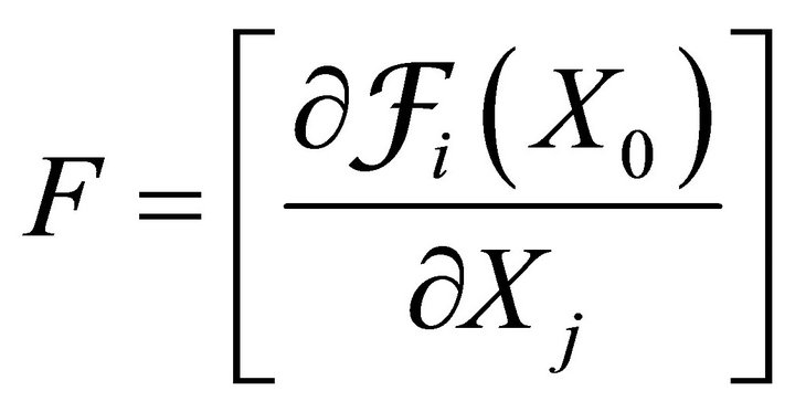 and
and 
where i = 1, 2; j = 1, 2.
Therefore,
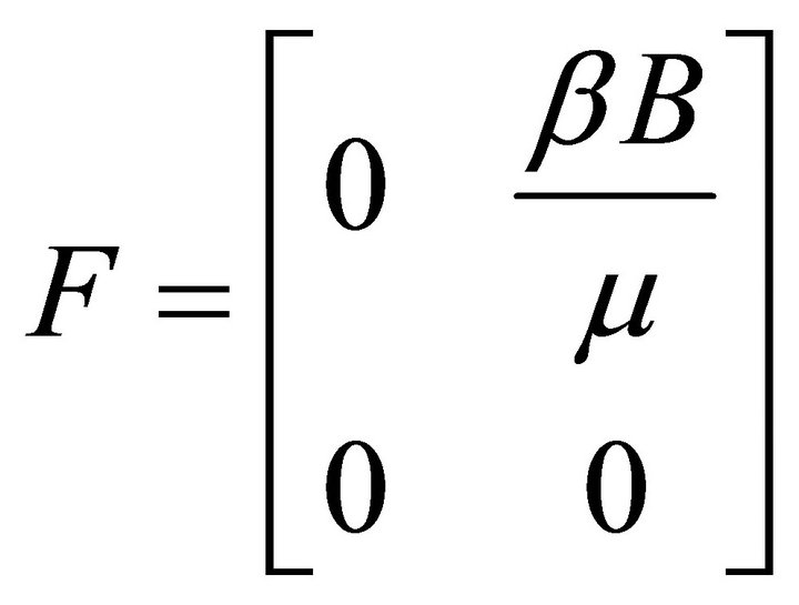 and
and 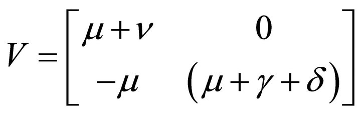
Here, V is a non-singular M-matrix. Therefore it is invertible. So,
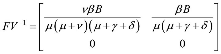
Hence, basic reproduction number R0 is given by

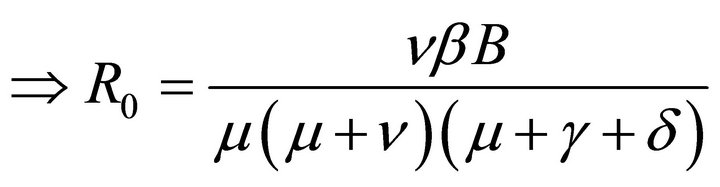 (5)
(5)
The disease free equilibrium  is locally asymptotically stable if all the eigenvalues of the matrix
  have positive real parts.
Theorem: Consider the disease transmission model given by (2) with . If
. If  is a disease free equilibrium of the model, then
  is locally asymptotically stable if
 , but unstable if
 , where
  is defined by (5).
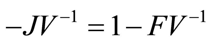
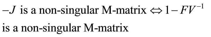
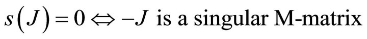
Proof: Let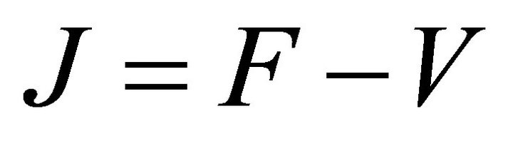 . Since V is a non-singular Mmatrix and F is non-negative,
 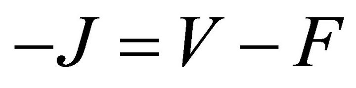 has the Zsign pattern. Thus,

{s(J) is spectral abscissa of J}.
Since  is non-negative,
 also has the Z-sign pattern.
Then, we have
Finally, since  is non-negative, all eigenvalues of
 have magnitude less than or equal to
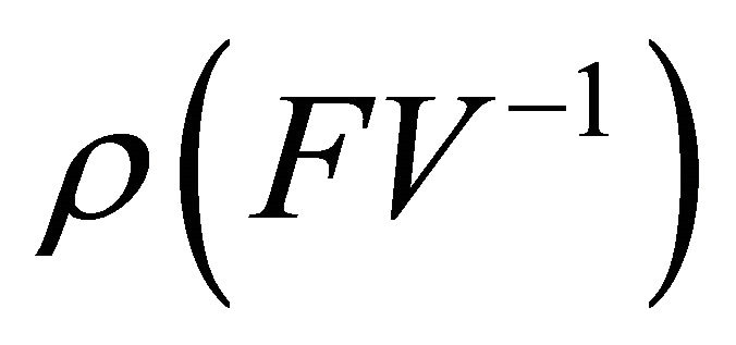 .
.
Thus,  is a non-singular M-matrix
 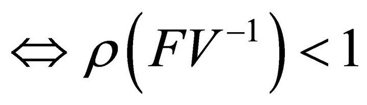 .
.
Hence,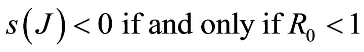 .
.
Similarly it follows that
 .
.
 .
.
Hence, .
.
It follows that
 .
.
 (5)
(5)
The disease free equilibrium  is locally asymptotically stable if all the eigenvalues of the matrix
have positive real parts.
3. Application to Vector Borne Disease
Now we apply this SEIR model to vector borne diseases especially in our case to malaria. The model is formulated for both—human population as well as vector population. At time t, for human population, there are Sh susceptible, Eh exposed, Ih infectious, Rh recovered and for vector population there are Sv susceptible, Ev exposed and Iv infectious. We do not take recovered class for vector population because once infected, mosquitoes are assumed to remain so until death.
The state variables and parameters used for two populations are listed below:
§ Mosquito Population
§ Sv: Number of susceptible mosquitoes;
§ Ev: Number of exposed mosquitoes;
§ Iv: Number of infectious mosquitoes;
§ Bv: Recruitment as susceptible per unit time;
§ ív: Rate of progression of mosquitoes from the exposed state to the infectious state;
§ σv: Mosquito biting rate;
§ ìv: Natural death rate;
§ pv: Probability of transmission of infection from an infectious human to a susceptible mosquito;
§ βv: Infection rate = pv ×σv.
§ Human Population
§ Sh: Number of susceptible humans;
§ Eh: Number of exposed humans;
§ Ih: Number of infectious humans;
§ Rh: Number of recovered humans;
§ Bh: Recruitment as susceptible per unit time;
§ íh: Rate of progression of humans from the exposed state to the infectious state;
§ βh: Removal rate;
§ äh: Disease-induced death rate;
§ ìh: Natural death rate;
§ ph: Probability of transmission of infection from an infectious mosquito to a susceptible human;
§ βv: Infection rate = ph ×σv.
Now the systems differential equations for both the populations describing the spread of malaria are as follows:
For human population
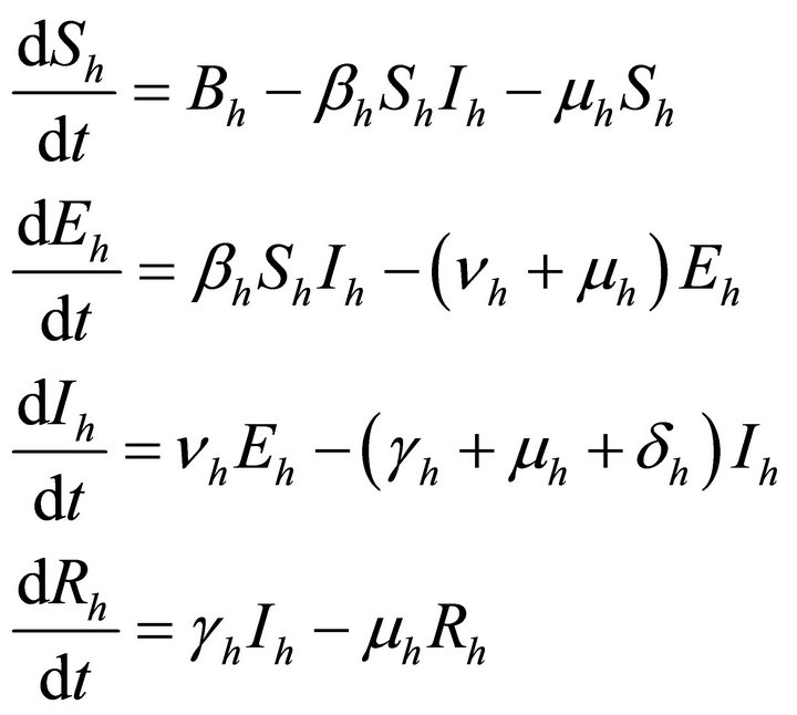 (6)
(6)
and for mosquito population
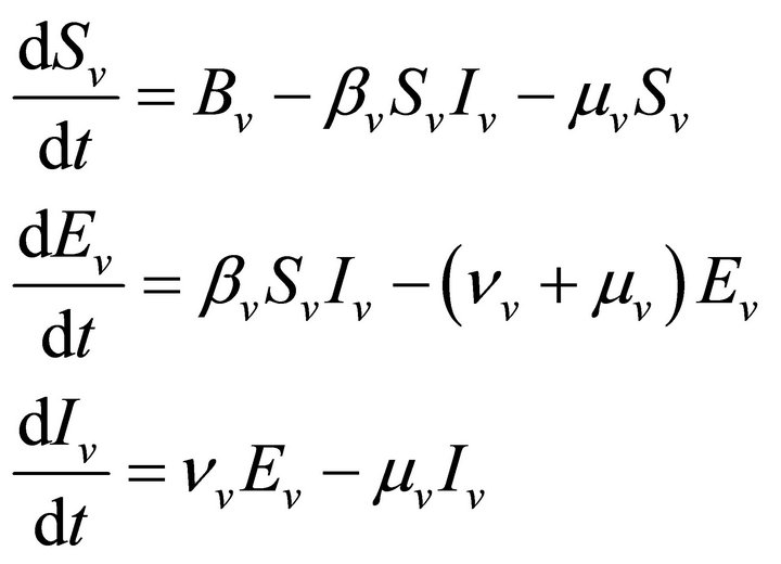 (7)
(7)
By relation (5), R0 is given by
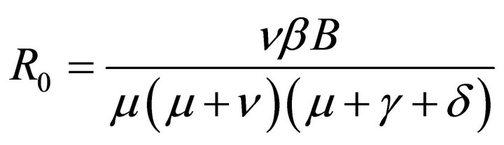
This shows that it is a product of the rate of production of 1) new exposures and 2) new infections.
Now if we have a system in which there are multiple discrete types of infected individuals [e.g. human and mosquitoes, men and women, human and chickens etc.], we define the next generation matrix as the square matrix G [6] in which ijth—element of G, gij is the expected number of secondary infections of type i caused by a single infected individual of type j assuming that the population of type i is entirely susceptible. That is, each element of the matrix G is a reproduction number, but one where who infects whom is accounted for.
So, in our case, there are two classes of infected individuals viz. human and mosquitoes. The next generation matrix is thus 2 × 2.
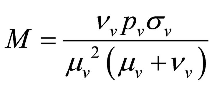
Let M be the expect number of infected mosquitoes and H be the expected number of infected humans given that the contact between the two occurs in completely susceptible population. Then the next generation matrix is
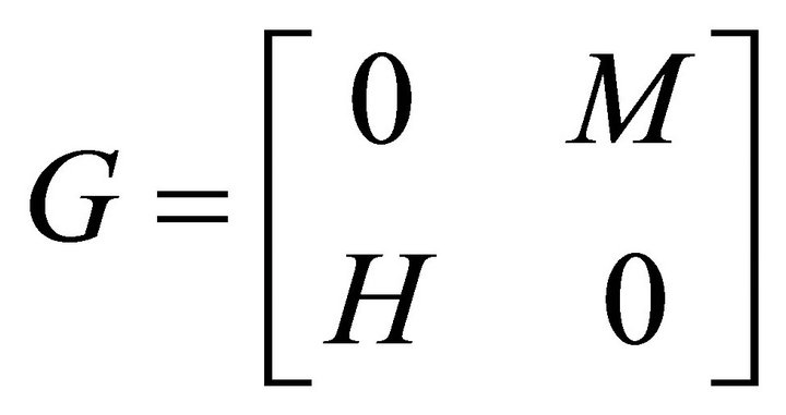
 (8)
(8)
where
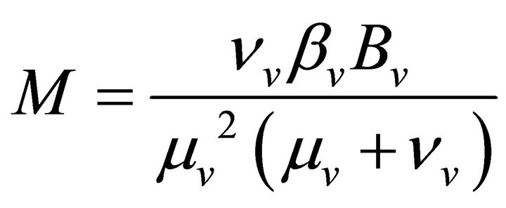 (using relation (5))
Here we analyse the model for epidemic situation, so new recruitments will not be allowed. So,
 and
and

Therefore, 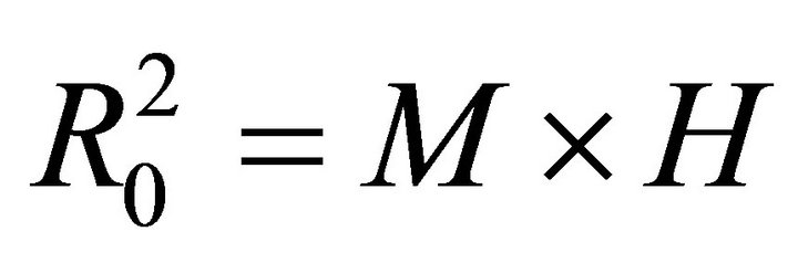
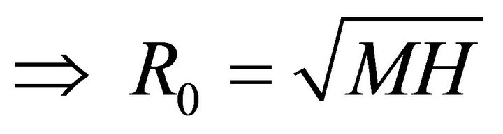
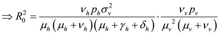 (9)
(9)
4. Sensitivity Analysis
In order to decide the most sensitive parameters, it is necessary to know the relative importance of the different factors responsible for its transmission. We calculate the sensitivity indices of R0 to the different parameters in the model. These indices tell us how crucial each parameter is to disease transmission.
Here, we use the normalised forward sensitivity index of a variable, u, which depends continuously on a parameter, p is defined as
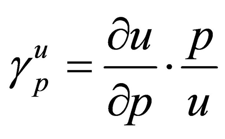
From Table 2, we see that the most sensitive parameters are mosquito biting rate σv and mosquito death rate μv.
5. Numerical Simulation
We do computer simulation using MATLAB for human population as well as for mosquito population to visualize the trends in each compartment.
6. Results and Discussion
Here we started with the basic SEIR epidemic model. We explained the basic assumptions made for formulating this model. A threshold parameter known as basic reproduction number, R0, is defined and a relation is derived for its calculation. It is shown that if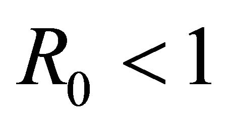 , then the disease free equilibrium is locally asymptotically stable whereas if
 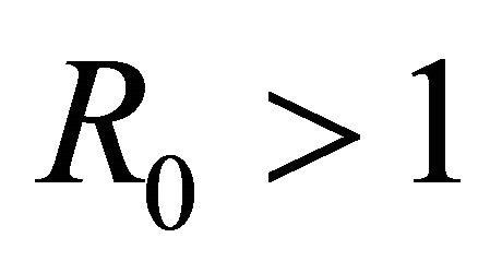 then it is unstable.
This theory is further applied to a vector borne disease namely malaria. SEIR model is formulated for both human as well as for vector population. Analysis is done for the combined effect of both the populations when the malaria is in epidemic state.
Sensitivity analysis shows that the most sensitive parameters are mosquito biting rate and mosquito death rate.
Simulation results show that in epidemic situation, both the populations will get almost completely infected within the two weeks of disease outbreak. Population does not remain in exposed compartment for long. This way, the results are helpful in predicting disease trends and so planning the right control actions and strategies.
7. Acknowledgements
The authors are thankful to reviewers for their constructive suggestions. This research is supported by UGC project scheme #41-138612012(SR).
REFERENCES
- J. Nedelman, “Introductory Review: Some New Thoughts about Some Old Malaria Models,” Mathematical Biosciences, Vol. 73, No. 2, 1985, pp. 159-182. doi:10.1016/0025-5564(85)90010-0
- J. L. Aron, “Mathematical Modelling of Immunity to Malaria,” Mathematical Biosciences, Vol. 90, No. 1-2, 1988, pp. 385-396. doi:10.1016/0025-5564(88)90076-4
- G. A. Ngwa and W. S. Shu, “Mathematical Model for Endemic Malaria with Variable Human and Mosquito Populations,” 1999. http://www.ictp.treste.it
- S. A. Al-Sheikh, “Modeling and Analysis of an SEIR Epidemic Model with a Limited Resource for Treatment,” Global Journal of Science Frontier Research: Mathematics and Decision Sciences, Vol. 12, No. 14, 2012, pp. 57- 66.
- P. van den Driessche and J. Watmough, “Reproduction Numbers and Sub-Threshold Endemic Equilibria for Compartmental Models of Disease Transmission,” Mathematics Biosciences, Vol. 180, No. 1-2, 2002, pp. 29-48. doi:10.1016/S0025-5564(02)00108-6
- J. H. Jones, “Notes on R0,” Stanford University, Stanford, 2007.
- C.-M. Dabu, “MATLAB in Biomodeling,” In: C. Ionescu, Ed., MATLAB: A Ubiquitous Tool for the Practical Engineering, InTech, Croatia, 2011.
- O. Diekmann and J. A. P. Heesterbeek, “Mathematical Epidemiology of Infectious Diseases: Model Building, Analysis and Interpretation,” Wiley, New York, 1999.