Applied Mathematics
Vol.3 No.12A(2012), Article ID:25985,6 pages DOI:10.4236/am.2012.312A279
Four Common Properties of Repairable Systems Calculated with the Boltzmann-Like Entropy
1IBM, Roma, Italy
2LUISS University, Roma, Italy
3Institute of Applied Mathematics Far Eastern Branch of RAS,
Vladivostok, Russia
Email: procchi@luiss.it, guram@iam.dvo.ru
Received September 7, 2012; revised October 7, 2012; accepted October 14, 2012
Keywords: Repairable System; Boltzmann-Like Entropy
ABSTRACT
Gnedenko, the father of the modern Reliability Theory, first derived some fundamental properties of reliable systems following rigid deductive logic. This paper shares the deductive method and infers four principal properties of repairable/maintainable systems using the Boltzmann-like entropy. In particular we calculate the reparability function and next discuss the physical meanings of the formal results. Lastly we comment on the broad range of applications and researches which can relate to this study.
1. Introduction
Boris Vladimirovich Gnedenko widely considered the founder of the modern Reliability Theory, deduces significant result on the basis of general hypotheses [1]. For instance the survival function was defined in biology as an empirical law; instead Gnedenko derives the reliability function by means of deductive logic. The present paper goes on this way. In particular we mean to calculate the effects of repairs and maintenance processes under general assumptions. This work follows two articles previously published on the same vein of research [2, 3].
We use the Boltzmann-like (or stochastic) entropy which quantifies the degree of reversibility of a system state. The meaning of the entropy may be intuitively introduced in the following terms. When the physical system works steadily, the functioning state is stable namely the system takes on a somewhat irreversible functioning state. When the system becomes unreliable, it frequently leaves the functioning state and the reversibility of the functioning state rises up. Other comments on the Boltzmann-like entropy follow in Section 3.
This research means to derive four properties of repairable systems through two steps: Section 2 develops the calculations and Section 3 comments on the physical meaning of the mathematical results.
2. Four Properties of the Repairability Function
2.1. Assumptions and Basic Definitions
We assume that S is a continuous time and discrete-state stochastic system:
 (1)
(1)
where  is the functioning or steady state during which the system runs;
  is the recovery state during which the system is repaired, or renewed etc. We assume Af and Ar are mutually exclusive
 (2)
(2)
We define  as the Boltzmannlike or stochastic entropy of the generic state Ai. The stochastic entropy is continuous increasing function defined in the codomain
 . As special cases we have that the reliability entropy of the state Af is
 ; and the recovery entropy of Ar is
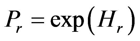
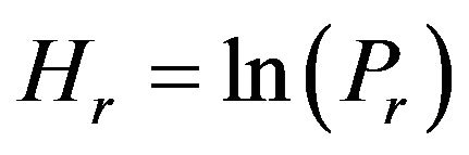 [2]. We obtain the probability of the recovery state Pr from the recovery entropy
 (3)
(3)
And get the probability Pf from (2)
 (4)
(4)
We calculate the reliability entropy in function of the recovery entropy (Figure 1) which we define as the reparability function
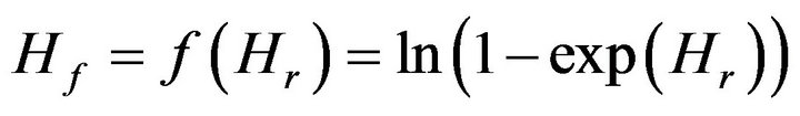 (5)
(5)
2.2. Property A
Denote
 (6)
(6)
Consider the cases i) , ii)
, ii)  using Taylor expansions. In case i) we have
 (7a)
(7a)
In case ii) we have
 (7b)
(7b)
Limits (7a) and (7b) yield the asymptotes
 (8)
(8)
2.3. Property B
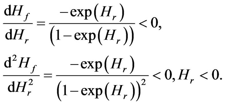
Using the formula (5) it is easy to obtain that
 (9)
(9)
This means that in turn (9) the functions
 both decrease continuously and monotonously from 0 to –∞ when the variable steps up from Hr = −∞ to Hr = 0. So for any h < 0 there is single
  so that
 (10)
(10)
Consequently we may choose h< 0, h< 0 so that  is sufficiently small and
  is sufficiently large and find zones
 (11)
(11)
In the zone α which characterizes asymptote Hf = 0 we have the inequality
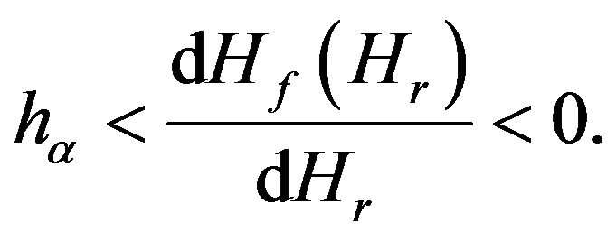 (12)
(12)
In the zone γ which characterizes asymptote Hr = 0 we have the inequality
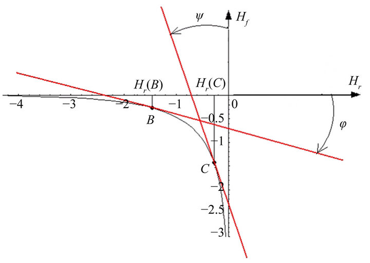
Figure 1. Special values of hα and hγ.
 (13)
(13)
2.4. Special Values of hα and hγ
Suppose that:
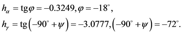 (14)
(14)
Then using (10) we have that coordinates of points B, C in Figure 1 are
 (15)
(15)
2.5. Property C and D
Put
 (16)
(16)
and introduce the finite difference
 (17)
(17)
From the formula (17) we have that
 (18)
(18)
consequently
 (19)
(19)
The formula (19) means that absolute value of the finite difference  is very small if
 ![]() and very large if
and very large if 
3. Physical Interpretation
We discuss the physical phenomena underlying the formal results obtained in the previous section.
3.1. Definitions: What the Entropy Function Calculates
By definition the stochastic entropy quantifies the reversibility and the irreversibility of each state of S and in consequence H depicts the physical behavior of a system. Let see the conduct of S in detail.
- The more the reliability Pf is high, the more Hf is high, and the more the functioning state Af is irreversible namely S works steadily in the world. The system does not leave Af in that S does not need to be restored. On the other hand the more S is unreliable, the more Af is reversible, and the more frequently S abandons the operating state Af as S is unreliable.
- The recovery entropy calculates the irreversibility of the recovery state, this implies that the more Hr is high, the more Ar is stable and in practice S is hard to be repaired and/or maintained in the physical reality. A low value of Hr means the Ar is reversible and S can be easily restored/maintained.
In sum the functions Hf. and Hr specify the behavior of S in the states Af and Ar respectively, instead Pf and Pr are the probabilities of each state. The meanings of the variable P and of the function H widely differ. The reliability and recovery entropies specify the grades of each state and describe the continuous modification of a system. The reliability entropy and the recovery entropy do not revolve around an “all or nothing” type of failure criterion.
3.2. Assumption: Artificial and Biological
Artificial systems perfectly comply with assumption (2), hence the properties of the reparability function apply to machines and devices in any detail.
Biological systems do not stop to leave when they are cured but the metabolism slows down. Some biological functions become feebler or even suspend during sickness. The states Af and Ar of biological systems do not switch in a perfect manner, but conform to (2) in a approximate manner; hence biological systems cannot follow the reparability function with precision, but they follow the most evident properties—A and C (partially)—which we are coming to comment on.
3.3. Property A: A Rule Relates the Performances of a System to Its Reparability
One interprets (7a) and (7b) using remarks 4.1 namely (7a) holds that a reliable system is easily repaired and (7b) proves that an unreliable system is repaired with efforts. e.g. an appliance that has low performances and frequently breaks down is uneasy to restore because—for example—there are several parts that should be replaced. Modern literature agrees that (7a) is typical of new systems and (7b) is typical of old systems.
Two features which appear independent in point of logic—the effectiveness and the reparability of a system—are strictly related by means of a rule.
• 3.4. Property B: A Repairable System Can Reach Three Main Levels of Quality
• Limits (7a) and (7b) hold that the domain of  does not include the extremes. The fully functioning system A that is never repaired and the irrecoverable system D do not pertain to the effects calculated by the reparability function. All the same the paradoxical states A and D are highly significant in the present theoretical frame. These extremes depict two situations similar to the ideal cases studied in mature disciplines such as mechanics, chemistry and electronics. For example the ideal gas obeys Boyle’s law exactly at all temperatures and pressures, and has internal energy that depends only upon the temperature. This ideal gas does not exist in the world nonetheless it is a fundamental reference in thermodynamics as a real gas may get more or less close to the ideal gas. In parallel we see that a real system S is more or less close to A and to D. We can but regard these extremes as models of excellence: the former is perfectly running the latter is absolutely irreparable. We define A and D as ideal cases of repairable/maintainable systems. We formally denote the upper and lower boundaries A and D with the terms “new system” and “old system” in accordance to current literature.
• Because a real system is located more or less close to an ideal case, we have to answer: How can be the proximity of a real system to the ideal system calculated?
• We adopt an empirical criterion which is familiar to experimentalists. They are aware that the measured quantity Ỹ may be affected by systematic errors. The value Ỹ can differ significantly from the expected value Y. Experimentalists assume the ensuing criterion to credit a measured quantity: Ỹ conform to Y if the gap between Y and Ỹ does not exceed 10% of Y
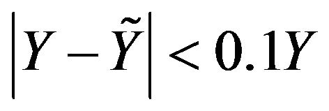
For example the expected value of a current is +70 volt, if the measure Ỹ falls inside +63 volt and +77 volt, than Ỹ may be associated to Y, otherwise is Ỹ discarded.
We have applied this empirical criterion to ascertain the quality of a real system and have got Equations (14) and (15).
The asymptote Hf = 0 is the tangent of the extreme A and forms a straight angle with the axe Hr. The straight angle is 180˚ thus 18˚ is the maximum deviation angle for the tangent of a point that can be reasonably associated to A. We call B the point whose tangent makes the maximum angle φ with the axis Hr

And C has the tangent that makes the maximum angle ψ with the axis Hf

The points of the interval (A, B) make the zone α and (C, D) makes γ Figure 2); and we can define the system which falls in α, as a system as-good-as-new (AGAN) and the system which falls in γ as-bad-as-old (ABAO). The coordinates of B and C prove that the terms “asgood-as-new” and “as-bad-as-old” denote contrasting degrees of effectiveness and reparability.
The horizontal zone α and the vertical zone γ of the reparability function are separated by the intermediate range β which (15) proves to be rather small in size. Assuming the distribution of the physical systems is uniform along the curve , the systems placed in β should be judged as a minority group. This conclusion matches with the professional practice that normally assigns a repaired system to AGAN or otherwise to ABAO, and ignores intermediate results.
3.5. Property C: Identical Repair Processes Can Result in Different Effects
The intervals ΔHf and ΔHr calculated with the reparability function make explicit the effects of a physical intervention on S. In detail ΔHf that quantifies the variation of the system performances is positive when S works better after the intervention; at the same time ΔHr is negative in

Figure 2. Evolution after the repair process.
fact S is better adjustable after the intervention. On the other hand positive ΔHr and negative ΔHf mean that the operating conditions become worse than the conditions observed prior to the restore/maintenance operations. In conclusion an intervention can bring forth positive or even negative effects.
We mean to discuss the effects of repair/maintenance in greater details using the reparability function.
Let the system is placed in α or in γ. When (16) true, the constant  refers to a well defined repair activity occurred in the physical reality, e.g. workers replace an old component of S with a new component. Quantities Q and q give the different improvements of performances after the repair k obtained respectively when a system is good-as-new or bad-as-old. In particular equations from (18) to (20) mean that the repair executed on effective systems carries on a negligible variation of the system performances; instead the same repair operated on an unreliable system results in significant improvements. e.g. the new component M that replaces the AGAN component M1 brings forth a little amelioration, instead M results in great amelioration when M replaces the very old component M2.
3.6. Property D: Four Types of Results in Repair/Maintenance
Suppose the system lays in the range γ, say close to X. We have the following typology of repairs/maintenance:
1) The system migrates in the range A-B and becomes as good-as-new. This result means that the repair or maintenance is perfect.
2) The system migrates in the range B-C and has intermediate quality. A treatment restores the system operating state to be somewhere between as good as new and as bad as old. This result means that the repair or maintenance is imperfect.
3) The system remains in the zone γ. This result means that S is still bad-as-old and the repair is minimal.
4) The system falls below X. Worse repair/maintenance damages the system status. The system’s operating condition becomes worse than that just prior to its failure.
Types from 1 to 4 exhaust the forms of repairs illustrated in current literature.
4. Conclusive Remarks
This paper applies the deductive logic using the Boltzmann-like entropy and finds out common properties A, B, C and D of repairable systems. In the first stage of Section 2 we prove that two features which appear independent in point of logic—the performances and the reparability of systems—are strictly related. As second we show how repairable/maintainable systems reach an infinite set of states which basically have two levels of quality: AGAN and ABAO. Thirdly we infer that a preventive/corrective intervention can bring different improvements in new and old systems; and lastly we deduce the processes called perfect, imperfect, minimal and worse repairs.
Current literature recognizes the laws (7a) and (7b) on the basis of indisputable empirical evidences in the technical and biological areas as well and generically relates this phenomenon to aging. Authors agree that (7a) describes devices recently produced and controlled in factories [4]; (7b) depicts the behavior of appliances running from long time. Property A has broader significance as it has not been derived from aging; the feature A can be originated by aging and even by other root-causes.
One important research area in reliability engineering is the study of various maintenance policies in order to prevent the occurrence of system failure in the field and to improve system availability [5]. Brown-Proschan [6] established the seminal model for imperfect repair. Later authors proposed a multitude of approaches and strategies. We quote Lie-Chun [7], Block-Borges-Savits [8], Whitaker-Samaniego [9], The vast majority of these studies assume that the system S becomes either asgood-as-new or as-bad-as-old after corrective recovery or preventive maintenance. Authors take AGAN and ABAO as mutually exclusive states notably S becomes AGAN with probability p and becomes ABAO with probability ; this is sometimes called the
  rule. The present paper refines these empirical conclusions and demonstrates that a system just repaired can assume infinite degrees of qualities. Besides the zones α and γ that are the most important, the reparability function brings evidence of the small zone β in accordance to Malik’s work who considers an intermediate degree of quality between AGAN and ABAO [10]. The ancillary role of β even matches with economical studies. The systems placed in β do not show significant edges in the sense that they do not guarantee perfect operating functions such as AGAN systems, neither the systems in β offer economical advantages like the ABAO systems whose restoration is cheap.
The present study proves how biological systems do not adhere to hypothesis (2) in a perfect manner (see 3.2) and in consequence medicine complies with Property A in generic terms. Physicians recognize the good response of young individuals to medical treatments, and how cures are far less effective for old patients [11], but the zones α and γ appear rather fuzzy to calculate in medicine. Doctors cannot tackle a systematic discussion of the curableness/incurableness of people. Actually gerontologists attack a broad spectrum of diseases and problems specific to old people on the basis of empirical researches [12]. As an example one can see the survival rates of
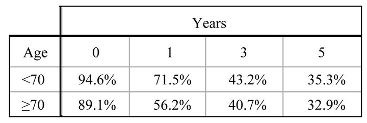
Figure 3. Survival rates.
elderly and younger patients who underwent esophageal resection [13] (Figure 3). The first column exhibits postoperative rate that is the percentage of all patients who did not die within 60 days after operation. The second, third and fourth columns display the survival rates Registered after 1, 3 and 5 years. The values of the older group are constantly higher than the values of the younger patient group, but one cannot deduce a rigorous rule.
Medical literature recognizes Property C, in particular the perfect restore is called “restitutio ad integrum” (= restitution in full). The sick man has become a perfect healthy person and does not miss any organ or even any small part of his body.
REFERENCES
- B. V. Gnedenko, Yu. K. Beliaev and A. D. Soloviev, “Mathematical Methods in Reliability Theory,” Science, Moscow, 1965.
- P. Rocchi, “Boltzmann-Like Entropy in Reliability Theory,” Entropy, Vol. 4, No. 5, 2002, pp. 142-150.
- P. Rocchi, “Calculations of System Aging through the Stochastic Entropy,” Entropy, Vol. 8, 2006, pp. 134-142.
- V. L. Bengtson, D. Gans, N. Putney and M. Silverstein, “Handbook of Theories of Aging,” Springer, Berlin, 2008.
- H. Z. Wang, “A Survey of Maintenance Policies of Deteriorating Systems,” European Journal of Operational Research, Vol. 139, No. 3, 2002, pp. 469-489.
- M. Brown and F. Proschan, “Imperfect Repair,” Journal of Applied Probability, Vol. 20, No. 4, 1983, pp. 851-859.
- C. H. Lie and Y. H. Chun, “An Algorithm for Preventive Maintenance Policy,” IEEE Transactions on Reliability, Vol. 35, No. 1, 1986, pp. 71-75. doi:10.1109/TR.1986.4335352
- H. W. Block, W. S. Borges and T. H. Savits, “A General Age Replacement Model with Minimal Repair,” Naval Research Logistics, Vol. 35, No. 5, 1988, pp. 365-372.
- L. R. Whitaker and F. J. Samaniego, “Estimating the Reliability of Systems Subject to Imperfect Repair,” Journal of American Statistical Association, Vol. 84, No. 405, 1989, pp. 301-309. doi:10.1080/01621459.1989.10478770
- M. A. K. Malik, “Reliable Preventive Maintenance Policy,” AIIE Transactions, Vol. 11, No. 3, 1979, pp. 221- 228.
- W. H. Cole, “Operability in the Young and Aged,” Annals of Surgery, Vol. 138, No. 2, 1953, pp. 145-157. doi:10.1097/00000658-195308000-00001
- J. M. Wilmoth and K. F. Ferraro, “Gerontology: Perspectives and Issues,” Springer, Berlin, 2006.
- S. Kinugasa, M. Tachibana, H. Yoshimura, D. Kumar Dhar, M. Shibakita, S. Ohno, H. Kubota, R. Masunaga and N. Nagasue, “Esophageal Resection in Elderly Esophageal Carcinoma Patients: Improvement in Postoperative Complications,” Annals of Thoracic Surgery, Vol. 71, No. 2, 2001, pp. 414-418. doi:10.1016/S0003-4975(00)02333-X