Applied Mathematics
Vol. 3 No. 5 (2012) , Article ID: 19050 , 7 pages DOI:10.4236/am.2012.35063
Legendre Approximation for Solving Linear HPDEs and Comparison with Taylor and Bernoulli Matrix Methods
Department of Applied Mathematics, School of Mathematical Sciences, Ferdowsi University of Mashhad, Mashhad, Iran
Email: emrantohidi@gmail.com, etohidi110@yahoo.com
Received March 10, 2012; revised April 6, 2012; accepted April 13, 2012
Keywords: Legendre Operational Matrix of Differentiation; Hyperbolic Partial Differential Equations; Legendre Polynomial Solutions; Double Legendre Series
ABSTRACT
The aim of this study is to give a Legendre polynomial approximation for the solution of the second order linear hyperbolic partial differential equations (HPDEs) with two variables and constant coefficients. For this purpose, Legendre matrix method for the approximate solution of the considered HPDEs with specified associated conditions in terms of Legendre polynomials at any point is introduced. The method is based on taking truncated Legendre series of the functions in the equation and then substituting their matrix forms into the given equation. Thereby the basic equation reduces to a matrix equation, which corresponds to a system of linear algebraic equations with unknown Legendre coefficients. The result matrix equation can be solved and the unknown Legendre coefficients can be found approximately. Moreover, the approximated solutions of the proposed method are compared with the Taylor [1] and Bernoulli [2] matrix methods. All of computations are performed on a PC using several programs written in MATLAB 7.12.0.
1. Introduction
In real world, many fundamental laws of physics and chemistry can be formulated as differential equations. In biology and economics, differential equations are used to model the behavior of complex systems. The mathematical theory of differential equations first developed together with the sciences where the equations had originated and where the results found application. However, diverse problems, sometimes originating in quite distinct scientific fields, may give rise to identical differential equations. Whenever this happens, mathematical theory behind the equations can be viewed as a unifying principle behind diverse phenomena.
As a powerful Mathematical tool for modeling many of natural models in applied sciences, one can refer to partial differential equations (PDEs). In mathematics, a PDE is a differential equation that contains unknown multivariable functions and their partial derivatives. PDEs are used to formulate problems involving functions of several variables, and are usually difficult to solve. So it is necessary applying high accurate numerical methods.
PDEs can be used to describe a wide variety of phenomena such as sound, heat, electrostatics, electrodynamics, fluid flow, or elasticity. These seemingly distinct physical phenomena can be formalized identically in terms of PDEs, which shows that they are governed by the same underlying dynamic. Just as ordinary differential equations often model one-dimensional dynamical systems, partial differential equations often model multidimensional systems.
Hyperbolic partial differential equations (HPDEs), are one of the most important subclasses of PDEs. Many of the equations of mechanics are hyperbolic, and so the study of hyperbolic equations is of substantial contemporary interest. The solutions of hyperbolic equations are “wave-like.” If a disturbance is made in the initial data of a hyperbolic differential equation, then not every point of space feels the disturbance at once. Relative to a fixed time coordinate, disturbances have a finite propagation speed. They travel along the characteristics of the equation. This feature qualitatively distinguishes hyperbolic equations from elliptic and parabolic PDEs.
HPDEs can model the vibrations of structures (e.g. buildings, beams and machines) and are the basis for fundamental equations of atomic physics. Wave equation and Telegraph equation are typical examples of HPDEs. Telegraph equation is commonly used in signal analysis for transmission and propagation of electrical signals and also has applications in other fields (see [3] and the references therein). On the other hand, much attention has been given in the literature to the development, analysis and implementation for the numerical solution of second-order HPDEs, especially telegraph equations (see for example [4-7]).
Since the beginning of 1994, the Taylor, Chebyshev, Legendre, Bessel, Hermite, Lagurre and Bernstein matrix methods have been used by Sezer and his coworkers in several papers (see [1] and references therein) to solve linear differential (including HPDEs), Fredholm Volterra integro difference equations and their systems. Yet so far, to the best of our knowledge, a practical matrix method which based on Legendre polynomials have had few results for approximating the solution of linear HPDEs. This partially motivated our interest in such method.
In this paper, in the light of the above-mentioned methods and by means of the matrix relations between the Legendre polynomials and their derivatives, we develop a new approach called the Legendre approximation for solving the second-order linear HPDEs in the form
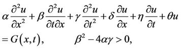 (1)
(1)
with the initial conditions
 (2)
(2)
and boundary conditions
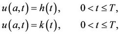 (3)
(3)
where  and
and  are constants. Without loss of generality and for clarity of presentation suppose that
 . Note that by a simple linear transformation these substitutions could be done.
Now, we assume that the solution of the considered HPDE is approximated as follows
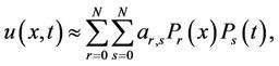 (4)
(4)
where  and
and  for all
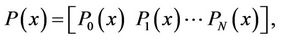
 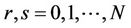 are the shifted Legendre polynomials in the interval [0,1] and the Legendre coefficients to be determined are
 .
.
The remainder of this paper is organized as follows: In the next section the Legendre polynomials together with their properties are introduced. Section 3 is devoted to presenting the Legendre operational matrix of differentiation in (one and) two dimensions, which is the fundamental section of the proposed method. In Section 4 we describe that how this matrix can be applied for solving the above-mentioned equation. Accuracy of the solution and error analysis are briefly discussed in Section 5. Illustrative examples are included in Section 6 for confirming the accuracy of the proposed approach. Finally conclusions are given in Section 7.
2. Legendre Polynomials
The Legendre polynomials which are orthogonal in the interval [–1,1] satisfy the following recurrence relation
 (5)
(5)
with 
In order to use these polynomials on the interval [0,1], one can apply the change of variables  in the above relation. Therefore, the shifted Legendre polynomials are constructed as follows
The orthogonal property of shifted Legendre polynomials is given by
 (6)
(6)
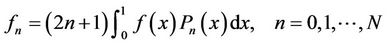
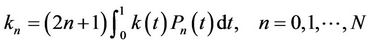
A function,  , which is absolutely integrable in the interval [0,1] may be expressed in terms of a shifted Legendre series as
 (7)
(7)
where
 (8)
(8)
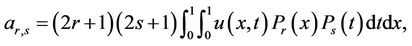
Moreover, by extending the above property in twovariable functions, one can conclude that if a (smooth enough) two variable function  be approximated by shifted Legendre polynomials in the form
 (9)
(9)
then, the coefficients  can be evaluated as follows

In the next section, we will introduce the operational matrix of differentiation of Legendre polynomials and then extend this matrix for two dimensional functions, which is called the two dimensional Legendre operational matrix of differentiation.
3. Two Dimensional Legendre Operational Matrix of Differentiation
The shifted Legendre polynomials have an interesting property (a relation between Legendre polynomials and their derivatives) which was used in many papers for solving different types of problems (see [8] and references therein). This relation is as follows
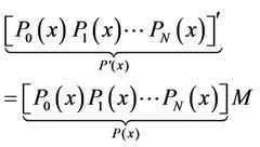 (10)
(10)
where
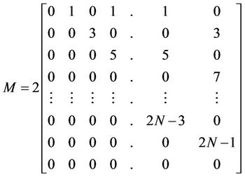
If N is even and

if N is even.
We recall that, M is the Legendre operational matrix of differentiation. Trivially for all positive integers
 , where our purpose from
  is the kth derivative of
Since in this paper we deal with two-variable functions, the above-mentioned matrix must be extended to a product of two matrices. Now, suppose that
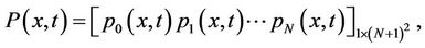 (11)
(11)
where 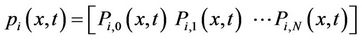 for all
 and
and for all
By a similar procedure that was used in [1], the relations between the matrix  and its derivatives are
 (12)
(12)
where  and
and
 ,
,

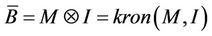
where our aim from  is the Kronecker product and I is the
  identity matrix.
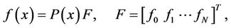
Now, consider the approximated solution (4), which can be rewritten in the matrix form
 (13)
(13)
where  is introduced in (11) and

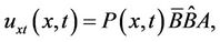
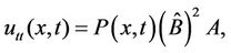
By using the relations (12) and (13), we have
 (14)
(14)
which are the fundamental relations of the proposed method. In the next section we describe our approach which is based on (14).
4. Method of the Solution
Our aim is to investigate the approximate solution of Equation (1), under the given conditions, in the series form of Equation (4) or in the matrix form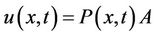 . To obtain the approximated solution, by using (14), we first reduce the terms of Equation (1) to matrix forms
 (15)
(15)
 (16)
(16)
 (17)
(17)
 (18)
(18)
 (19)
(19)
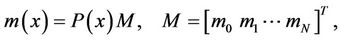
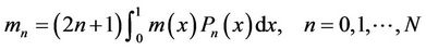
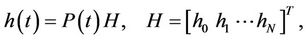
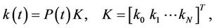
We can also approximate the function  in terms of Legendre polynomials as follows
 (20)
(20)
From (20),  can be represented in the matrix form
 (21)
(21)

Substituting the expressions (13), (15)-(19) and (21) into the basic Equation (1) and simplifying the result, we have the matrix equation
 (22)
(22)
Briefly, we can write Equation (22) in the form
 (23)
(23)

is the matrix coefficients.
We now present the alternative forms for  which are important to simplify matrix forms of the conditions. The simplification in conditions is done only with respect to the variable x or t. Therefore, we must use different forms for initial and boundary conditions. For initial conditions (2)
 (24)
(24)
and
 (25)
(25)
Also, for boundary conditions
 (26)
(26)
The matrix representations of non-homogeneous terms of Equations (2) and (3) can be written in the forms
 (27)
(27)
 (28)
(28)
 (29)
(29)

 (30)
(30)


By substituting relations (24)-(30) into Equations (2) and (3) and then simplifying the results, we get the matrix forms of conditions, respectively, as
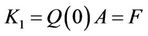
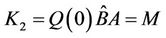

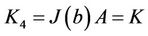
To obtain the solution of Equation (1) under conditions (2) and (3), the augmented matrix is formed as follows:
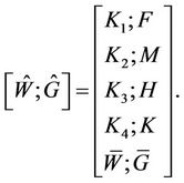 (31)
(31)
The unknown Legendre coefficients are obtained as
where  is generated by first using the Gauss elimination method to
  and then removing zero rows of the eliminated matrix. Here
  and
and  are obtained by throwing away maximum number of row vectors from
  and
and  so that the rank of the system that defined in (31) can not be smaller than
  This process provides higher accuracy because of decreasing truncation error.
5. Accuracy of the Solution and Error Analysis
We can easily check the accuracy of the method. Since the truncated Legendre series (4) is an approximate solution of Equation (1), when the function  and its derivatives are substituted in Equation (1), the resulting equation must be satisfied approximately; that is, for


If max  (
( positive integer) is prescribed, then the truncation limit
  is increased until the difference
  at each of the points becomes smaller than the prescribed
  On the other hand, the error can be estimated by
  and
and  errors and rootmean-square error (RMS). We calculate RMS error by the following formula [1]:
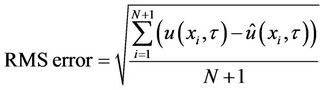
where  and
and  are the exact and approximate solutions of the problem, respectively and
  is an arbitrary time
  in
in 
6. Illustrative Examples
In this section, three examples are given to demonstrate the applicability, efficiency and accuracy of the proposed method. Each example is modeled using the mathematical software package MATLAB 7.12.0 and all calculations are run on a Pentium 4 PC Laptop with 2 GHz of CPU and 2 GB RAM.
Example 1. [9,10] Consider the following linear HPDE
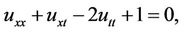
with the initial conditions
 and
and 
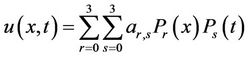
We assume that the problem has a solution in the form
 .
.
The fundamental matrix equation of this problem become
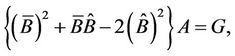
and this leads to the following solution
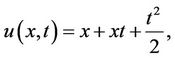
which is the exact solution.
In the following lines the MATLAB codes of this example are provided.
N=3;
format rat syms x t;
L1=zeros(1,N+1); L2=zeros(N+1,1);
L1=sym(L1); L2=sym(L2);
for i=1:N+1 L1(1,i)=poly2sym(shifted_logendre(i-1,0,1),x);
L2(i,1)=poly2sym(shifted_logendre(i-1,0,1),t);
end bb=zeros(N+1);
k=1;
for i=1:N+1 for j=1:i-1 k=i-j;
if k/2-fix(k/2)==0 bb(i,j)=0;
else bb(i,j)=2*(2*j-1);
end k=k+2;
end end Bb=zeros((N+1)^2);
Bb=kron((bb)',eye(N+1));
Bh=zeros((N+1)^2);
Bh=kron(eye(N+1),(bb)');
Q=zeros(N+1,(N+1)^2);
Q=kron(eye(N+1),subs(L1,x,0));
W=zeros((N+1)^2);WWW=zeros((N+1)^2);
WW=zeros((N+1)^2-2*(N+1),(N+1)^2);
W=(Bb)^2+Bb*Bh-2*(Bh)^2;
for i=1:(N+1)^2-2*(N+1)
for j=1:(N+1)^2 WW(i,j)=W(i,j);
end end WWW=vertcat(WW,Q,Q*Bh);
GG=zeros((N+1)^2-2*(N+1),1);GGG=zeros((N+1)^2,1);
F=zeros(N+1,1);M=zeros(N+1,1);
f=x;m=x;
for i=1:N+1 F(i,1)=(2*i-1)*int(f*L1(1,i),x,0,1);
M(i,1)=(2*i-1)*int(m*L1(1,i),x,0,1);
end GGG=vertcat(GG,F,M);
GGG(1)=-1;
A=inv(WWW)*GGG;
U=simplify(kron(L1,subs(L1,x,t))*A);
Example 2. Consider the following linear HPDE

with the initial
 and
and 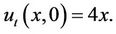
Similar to the first example, suppose that the problem has a solution in the form
 .
.
The fundamental matrix equation of this problem is

and this leads to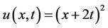 , which is the exact solution. Also, the readers can design a similar MATLAB codes for obtaining the exact solution of this example.
Example 3. [1,2] As the final example, consider the telegraph equation
under initial conditions
with the exact solution .
.
Following the procedure in Section 4, we find the fundamental matrix equation as follows

By taking different values of N, we solved the above problem by means of the fundamental matrix equation. The errors associated with the present method and Taylor method [1] together with the Bernoulli matrix method [2]
for N = 9 are compared in Table 1.
From this Table one can see that the associated errors of the Taylor method usually increase during the computational interval [0,1], meanwhile the Bernoulli [2] and the proposed methods have stable behaviors in this interval. With the experience of the author, the Taylor method have unstable behavior to dealing with long variation functions (such as exponential or hyperbolic functions) with regard to Legendre and Bernoulli method in the interval [0,1]. Moreover, outside the interval [0,1] the Legendre method again achieve to more accurate solutions with respect to the Taylor and Bernoulli methods. Also, we can consider more large intervals for showing the efficiency of the Legendre polynomials with respect to other polynomials such as Bernoulli etc. In addition the Taylor method obtain better solutions with respect to a multiwavelet method [1]; this issue support the efficiency of the proposed method.
Note that we use the shifted Legendre polynomials in the interval [0,2] instead of [0,1]. By doing this work, all of the available matrices divided by 2.
7. Conclusion
This article reports a matrix approach based on two-dimensional Legendre series for numerically solving linear HPDEs. Proposed method finds the Legendre series satisfying the conditions, and satisfying the differential equations by using an operational matrix of differentiation. This direct method avoiding any iterative procedure. One clear advantage of the presented method is that, once approximate the Legendre coefficients have been found, the approximate solution can immediately be evaluated at any point the range of integration. Computational results
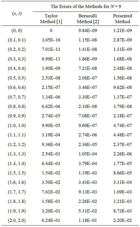
Table 1. Error comparisons of the presented method with taylor method [1] and bernoulli method [2] of example 3 for N = 9.
have been presented demonstrating the accuracy and reliability method. An estimation of the truncation limits is very important for the computational efficiency. If the truncation limit N is chosen too large, more work than necessary will have done. For this reason, the truncation limits must be chosen sufficiently large. The method is applied to all linear PDE and simple to use. We treat here two-dimensional problems only. However, it is straightforward to extend the method to more dimensions.
8. Acknowledgements
The author is grateful to the anonymous referee for a careful checking of the details and for helpful comments that improved this paper.
REFERENCES
- B. Bulbul and M. Sezer, “Taylor Polynomial Solution of Hyperbolic Type Partial Differential Equations with Constant Coefficients,” International Journal of Computer Mathematics, Vol. 88, No. 3, 2011, pp. 533-544. doi:10.1080/00207161003611242
- E. Tohidi and M. Shirazian, “Numerical Solution of Linear HPDEs via Bernoulli Operational Matrix of Differentiation and Comparison with Taylor Matrix Method,” Mathematical Science Letters, Accepted.
- M. Dehghan and A. Shokri, “A Numerical Method for Solving the Hyperbolic Telegraph Equation,” Numerical Methods for Partial Differential Equations, Vol. 24, No. 4, 2008, pp. 1080-1093. doi:10.1002/num.20306
- A. Ashyralyev and M. E. Koksal, “On the Numerical Solution of Hyperbolic PDE with Variable Space Operator,” Numerical Methods for Partial Differential Equations, Vol. 25, No. 5, 2009, pp. 1086-1099. doi:10.1002/num.20388
- F. Gao and C. Chi, “Unconditionally Stable Difference Schemes for a One-Space-Dimensional Linear Hyperbolic Equation,” Applied Mathematics and Computation, Vol. 187, No. 2, 2007, pp. 1272-1276. doi:10.1016/j.amc.2006.09.057
- R. K. Mohanty and M. K. Jain, “An Unconditionally Stable Alternating Direction Implicit Scheme for the Two Space Dimensional Linear Hyperbolic Equation,” Numerical Methods for Partial Differential Equations, Vol. 17, No. 6, 2001, pp. 684-688. doi:10.1002/num.1034
- R. K. Mohanty, M. K. Jain and U. Arora, “An Unconditionally Stable Adi Method for the Linear Hyperbolic Equation in Three Space Dimensions,” International Journal of Computer Mathematics, Vol. 79, No. 1, 2002, pp. 133-142. doi:10.1080/00207160211918
- R. K. Pandy, N. Kumar, A. Bhardwaj and G. Dutta, “Solution of Lane-Emden Type Equations Using Legendreoperational Matrix of Differentiation,” Applied Mathematics and Computation, Vol. 218, No. 14, pp. 7629- 7637.
- J. Biazar and H. Ebrahimi, “An Approximation to the Solution of Hyperbolic Equations by Adomian Decomposition Method and Comparison with Characteristics Method,” Applied Mathematics and Computation, Vol. 163, No. 2, 2005, pp. 633-638. doi:10.1016/j.amc.2004.04.005
- X. Yang, Y. Liu and S. Bai, “A Numerical Solution of Second-Order Linear Partial Differential Equations by Differential Transform,” Applied Mathematics and Computation, Vol. 173, No. 2, 2006, pp. 792-802. doi:10.1016/j.amc.2005.04.015