Modern Economy
Vol. 3 No. 1 (2012) , Article ID: 16797 , 7 pages DOI:10.4236/me.2012.31003
FDI and Employment by Industry: A Co-Integration Study
1Economics Philosophy, Dongbei University of Finance and Economics, Dalian, China
2Department of Economics and Management, Beijing Institute of Petrochemical Technology, Beijing, China
Email: lucyliuliyan@bipt.edu.cn
Received July 29, 2011; revised September 16, 2011; accepted October 20, 2011
Keywords: FDI; Employment by Industry; Co-Integration; ECM
ABSTRACT
The relationship between high levels of FDI and of employment has been of enduring interest in the development literature, particularly in the context of economy as China which has enjoyed exceptional inflows of foreign capital as well as huge amount of working population. Aiming at exploring the specific relations between FDI and employment of three strata industries in china, EG co-integration method and Granger causality test is applied to identify the long-run relations and short-run linkages between FDI and employment in each of the industry via distributed lag model; moreover, first-order and second-order ECMs are created to assess the short-term deviation. Findings indicate that, in secondary and tertiary industry, growth of FDI in the long run would promote employment, and it is especially true for tertiary industry, where bidirectional linkage between FDI and employment exists; in the short term FDI has limited and even negative impetus on employment, with the latter indirectly increasing the former.
1. Introduction
Since the economic reform and opening up policy, China has undergone remarkable economic development; concomitantly, there has been an enormous inflow of foreign direct investment (FDI) into the country. Indeed, China has now been one of the most attractive destinations for cross-border direct investment; and since 2000 China has become the world’s second largest recipient of FDI after the US. According to the world investment report [1], China attracted $560.39 billion US dollars of FDI for the period 1980 to 2004. It would seem to be a reasonable assertion that FDI made great contribution to both economic and employment growth of china. For example, in 2006 foreign funded enterprises accounted for 28 per cent of China’s added value in the industrial sector, exported about 58% of total exports of goods and services and imported 51% of total imports, and accounted for 11 per cent of local employment (China Investment Year Book (2006)).
Employment-generation or -promotion effect of FDI has attracted considerable attention, and some studies have been generated endeavored to explore the linkage between FDI and employment; earlier studies on the employment effect of FDI as Niu [2] found that FDI had a conspicuous positive impact on China’s employment growth when domestic investment efficiency was of low level or comparatively decreasing. Summon, Saul and Klaus [3] concluded that wholly-owned FDI operations had higher employment growth effect, while local industry characteristics moderate the growth effect; however, in the context of a more broad-based general equilibrium framework of employment, human capital, liberalization and openness, findings indicated that FDI had limited, even negative, impact on the Chinese economic growth and employment creation [4].
Another strand of literature addressed employment structure implications of FDI. Under the framework of human capital, Cai and Wang [5] studied the impact of FDI on China’s employment structure, distribution and labor market, concluded that FDI had a positive impact on the development of labor market and the accumulation of human capital. Zhang and Ren [6] focused particularly on the relations of FDI and employment structure, and found that FDI promoted China’s employment structure via the transition of rural labor to non-agricultural industries and the quality improvement of labor force.
Yet the definite conclusion of FDI’s impact on employment still remains disputed, and its specific linkage with three strata industry has not received enough attention in recent literature. Based on the real utilized FDI for the period 1985-2008, the purpose of this paper is to explore the specific relations between FDI and employment of three strata industry in the particular literature of china. The rest of the paper is organized as follows. Section 2 contains the details of measurements of variables. In Section 3, Section 3.1 gives background information of co-integration; Section 3.2 presents integration test for six series, where the MacKinnon EG co-integration critical value is high-lighted; and EG co-integration, Granger causality test are in Section 3.3. Section 4 moves to error correction model with associated statistics, equations and graphs. This section also settles the core issues for the paper. Finally, Section 5 contains summary and conclusions based on all the estimations.
2. Data Description
2.1. Definitions and Measurement
Three Strata of Industries (Primary Industry, Secondary Industry, and Tertiary Industry): Different from International Standard Industrial Classification of all Economic Activities (ISIC Rev.3), the three strata of industries in China follows Industrial classification for national economic activities (GB/T4754-2002)1. According to “Industrial Classification for National Economic Activities (GB/ T4754-2002)”, the industrial classification in Chinese national accounts is based on statistics and accounting data [7]. Specifics as follow: Primary industry includes sections as agriculture, forestry, animal husbandry and fishing; Secondary industry contains sections as industry, mining, manufacturing, production and distribution of electricity, gas and water, and construction; Tertiary industry involves all sections and divisions that are not covered by primary and secondary industry2.
FDI (Utilized Annual Value of FDI by Industry): FDI is measured as the value of FDI inflow. The utilized annual value of FDI inflow refers to the investment actually occurred each year. Since it takes time for capital transferring and equipment shipping, there usually is a gap between contracted FDI and actually utilized FDI each year, and utilized FDI should be more precise than its contracted value in determining its impact on employment.
Since the official statistics (China Statistics Year Book) for utilized FDI value by section only begins from 1997, and from 1985 to 1996 there is only the proportion of utilized FDI value by section. As for the utilized annual FDI value by section from 1985 to 1996, the author tried to construct utilized FDI series by section through multiplying the total annual utilized FDI with the proportion each section accounts for. And through the sum of the section series, three (primary, secondary and tertiary industry) time series of FDI by industry are created.
Employment (Number of Employed Persons at Yearend by Three Strata of Industry): annual average employment is used to measure labor force participation in economic activities. Employment is measured by annual number of persons employed at year-end by three strata of Industry.
2.2. Data on the Six Time Series
The annual data of utilized FDI by industry (1997-2008) and total annual utilized FDI (1985-2008) are collected and calculated from China Statistics Year Book, annual proportion of utilized FDI value of each section (1985- 1996) are collected from China Foreign Economic Statistical Year book. FDI inflows (originally in US Dollars) are converted into real domestic values by (annual average series of) RMB to US dollar exchange rate. The time series cover the year of 1985 to 2008. All variables are converted into logarithms in the estimation. The graph of the six variables, in their logarithmic values, is given in Figure 1.
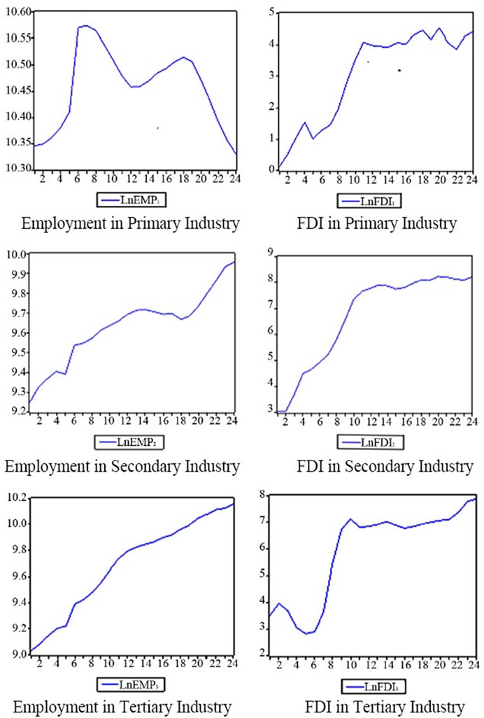
Figure 1. Six variables in logarithmic values.
3. The EG Co-Integration Method
3.1. Background
Equilibrium Theory in economics shows the existence of long-run equilibrium relation, indicating the adjustability of deviations from equilibrium caused by external influences and the recoverability of equilibrium through its future time periods, in the absence of any internal mechanisms to break the equilibrium.
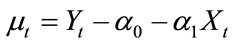
Assume that the long-run equilibrium relation between X and Y can be described as: Yt = α0 + α1Xt + μt (3.1), with μt denoting the disturbance term. If Xt is defined as X, then Yt shall be: α0 + α1X. At the end of time period t – 1, one of the followings will occur: 1) Y equals to its equilibrium value, Yt–1 = α0 + α1 t–1; 2) Y is smaller than its equilibrium value, t–1 < α0 + α1Xt–1; 3) Y is larger than its equilibrium value, Yt–1 > α0 + α1Xt–1.
Assumed X and Y are in its long-run equilibrium, and X changed in its value as ΔXt, then Y shall change correspondingly in its value as ΔYt:
 (3.2)
(3.2)
However, this is not always the case; the change of Y may be smaller or larger than its equilibrium value. To ensure the equilibrium in Equation (3.1), the difference between real changed value of Y and its equilibrium value ΔY must be stationary, meaning the disturbance term μt![]() I(0). Series μt is also named as disequilibrium error, the linear combination of X and Y:
I(0). Series μt is also named as disequilibrium error, the linear combination of X and Y:
 (3.3)
(3.3)
If X and Y are in long-run equilibrium (3.1), μt would be a stationary one with zero expected value: μt![]() I(0); and the two variables X and Y are of same-ordered, then X and Y can be called co-integrated. In its economic sense, co-integration statistically expressed the notion of equilibrium.
I(0); and the two variables X and Y are of same-ordered, then X and Y can be called co-integrated. In its economic sense, co-integration statistically expressed the notion of equilibrium.
For the two-variable co-integration test, the EngleGranger two-step method (null: random walk) [8] is widely used; in the following section, EG method is applied to test the existence of long term relations between employment and FDI in each industry.
3.2. Integration Test of the Six Series
Before checking the co-integrated relations between employment and FDI in the three industries, tests shall be taken to see whether the variables are of same order hence to avoid spurious regression estimations. For this reason, ADF (Augmented Dickey-Fuller Test, [9,10]) is performed to check the order of the variables.
For the constant and linear trend in ADF test, statisticcal significance of their coefficients is taken into consideration in determining whether to include them in the unit root tests; according to standard lag selection exclusion and lag length criteria, AIC (information criteria of Akaike-Schwarz), the lag structure for the ADF test is 2.
As shown in Table 1, ADF test alone shows all variables are I(1), save for lnEMP2 and lnFDI2, which are I(2). Since time series of lnEMP1 and lnFDI1 have same order of integration: (![]() I(1)), so do integration series of lnEMP2 and lnFDI2(
I(1)), so do integration series of lnEMP2 and lnFDI2(![]() I(2)), and lnEMP2 and lnFDI2 (
I(2)), and lnEMP2 and lnFDI2 (![]() I(1)); therefore it is eligible to further estimate the long run equilibrium relations (existence of co-integration) between employment and FDI in each industry.
I(1)); therefore it is eligible to further estimate the long run equilibrium relations (existence of co-integration) between employment and FDI in each industry.
3.3. EG Co-Integration Test and Granger Causality Test
3.3.1. EG Co-Integration Test
Follow the EG Co-integration test, OLS co-integrating regression as the first step will be performed to estimate the disequilibrium error:

The second step is to check whether residual series et is a stationary one (I(0) series) or not. According to (3.1) and (3.3), if Xt and Yt is co-integrated, the residual μt must be stationary.
As for the residual unit root test, DF or ADF unit root test can be applied; however, its critical value shall be quite different from that of ordinary one. Since the DF or ADF test is for the error series et in the integration equation, but not the real disequilibrium error μt in (3.1). Moreover, OLS estimation is based on the least total sum of squares, the estimator δ has a downward deviation, resulting in greater possibilities of refusing the null hypothesis. Therefore, critical values for the residual series

Table 1. ADF unit root test.
et shall be smaller than the usual critical values of DF and ADF test. For the residual unit root test, we shall follow the Engel-Granger co-integration critical values obtained through simulation tests held by MacKinnon [11,12]. The equation for critical values calculating is as:
Cp = φ¥ + φ1 T–1 + φ2 T–2, with the value of φ¥, φ1 and φ2 in Table 2.
Based on the equation and the surface response of critical values for co-integration test, the critical value for our particular co-integration test is –3.58697. And the Estimation equations for the three strata industry are as follows:
Primary industry:
 (3.4)
(3.4)
[287.851]*** [0.819]
R2= 0.030 DW = 0.296.
ADF unit root test for the residual series e1t in (3.4):
 (–2.07611)(3.5)
T-statistics is –2.076, and the 5% MacKinnon EngelGranger co-integration critical value3 is “–3.58697”, which shows strong evidence to accept null hypothesis, i.e. residual series e1t has a unit root, hence there is no longrun equilibrium relation between lnEMP1 and lnFDI1, which is generally consistent with the statistically insignificant R2 value. The result indicates impact of FDI on employment of primary industry is not statistically significant enough, which is explainable due to the lower technological quality of labor force in the industry and the technically sophisticated capital of FDI.
Secondary industry:
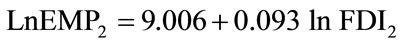 (3.6)
(3.6)
[151.548]*** [10.889]***
R2 = 0.844 DW = 0.393.
As approved in the foregoing integration test, lnEMP2 and lnFDI2 are I(2) series; therefore, residuals unit root test of their second-order difference series are as follow4:

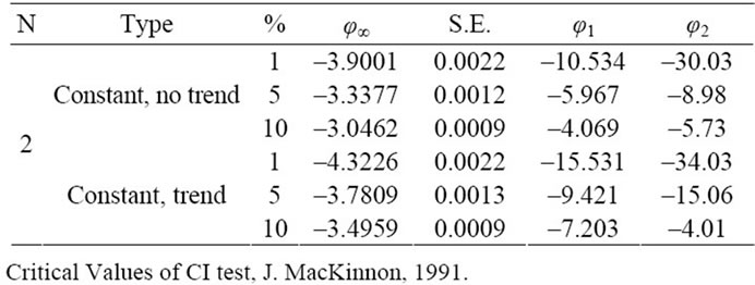
Table 2. Surface response of critical values.
[–3.7896]** (3.7)
The T-statistics for the residual unit root test is “–3.7896”, which is far lower than the 5% MacKinnon Engel-Granger co-integration critical value “–3.58697”; therefore, there is long term equilibrium relation between variables lnEMP2 and lnFDI2.
Tertiary industry:
 (3.8)
(3.8)
[74.968]*** [10.115]***
R2 = 0.823 DW = 0.434 ADF unit root test for the residual series et:
 [–3.977]***(3.9)
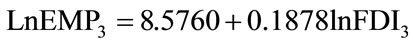
T-statistics is –3.9771, refusing the null hypothesis; hence we can draw the conclusion that the variables lnEMP3 and lnFDI3 are co-integrated.
3.3.2. Granger Causality Test
To further examine the specification of the possible linkages between the pairs of variables, it is necessary to perform the Granger causality test [13,14]. Since the precondition of the Granger causality test is that all the series shall be stationary or I(0) series, therefore, the nonstationary I(1) and I(2)series are differenced as ΔlnEMP3, ΔlnFDI3, and Δ2 lnEMP2, Δ2 lnFDI2, and lag length is automatically selected according to AIC (Akaike Information Criterion).
Results of Granger causality test in Table 3 indicates that in the secondary industry Δ2 lnFDI2 does Granger Cause Δ2 lnEMP2 (p-value is 0.02772, which refused the null hypothesis), while Δ2lnEMP2 does not Granger Cause Δ2 lnFDI2 (p-value is 0.572, which is great enough to accept the null hypothesis); while the case are quite different in the tertiary industry, which shows that ΔlnFDI3 does Granger Cause ΔlnEMP3 and vice versa. This bidirectional linkage between FDI inflow and employment implies the FDI-attracting capacity of the industry.
4. The Error Correction Model
Based on the long-run equilibrium and the Granger causality relations between FDI and employment in the secondary

Table 3. Pairwise granger causality tests.
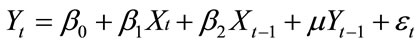
and tertiary industry, the short run relations will be tested. According to Granger representation theorem [15]: if variables Xt and Yt are co-integrated (Xt, Yt ![]() I(1)),then the short-run disequilibrium relation between Xt and Yt can always be described with an error correction model:
I(1)),then the short-run disequilibrium relation between Xt and Yt can always be described with an error correction model:
 (4.1)
(4.1)
μt denotes disequilibrium error or long-run deviation, and λ short-run regulation factor.
According to Error Correction Model (DHSY) [16], in real world, variables Xt and Yt are seldom in their long run equilibrium, and what people virtually observed is the short-run or disequilibrium relations as (with the hypothesis that there is first order distributed lag length):
 (4.2)
(4.2)
which shows that the value of variable Yt relates to both the change of Xt, and their respective values in their t – 1 time period.
To make the variables in the two sides of the equal mark stationary, Equation (4.2) can be transformed into:
Let  then
then
 . (4.3)
If we take the parameters α0, α1 (4.3) as identical with their corresponding ones in (4.2), Yt-1 = α0 – α1Xt–1 (4.3) will be the disequilibrium error in t – 1 time period. Then we get:
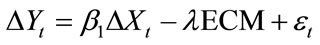 . (4.4)
Here ECM denotes the error correction term.
4.1. Secondary Industry
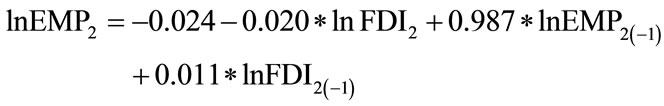
Since the long run relation between lnEMP2 and lnFDI2 has been explored as showed in (3.6):
 (4.5)
(4.5)
[151.548]*** [10.889]***
R2 = 0.844 DW = 0.393 From the value of DW (0.393), there is conspicuous series correlation between the two variables; hence simple lag equation is created as follow:
 (4.6)
(4.6)
[–0.020] [–0.564] [7.415]*** [0.345]
R2 = 0.953 DW = 2.021 LM(1) = 0.006 LM(2) = 0.360 LM(3) = 0.355 With the DW value as 2.02 and the F-statistics of LM test, series correlation has been diminished. And to further check the stationarity of the residuals :
:
[–4.670]***(4.6)
R2 = 0.509 DW = 1.989 LM(1) = 0.067 LM(2) = 0.318 The estimation of residual series shows that (4.5) is stationary; Figure 2 provides the graphs of the actual, fitted and residual values for (4.5). The virtual coincidence between the actual and fitted values is apparent for the equation. The early fluctuation phase of employment and its subsequent growth phase followed by a second fluctuation are almost perfectly tracked by the estimated Equation (4.5). Residual series being I(0) under the ADF test, with test statistics carrying a probability of nearly reaching zero.
Based on (4.5), second-order error correction model is created. Since lnEMP2![]() I(2), lnFDI2
I(2), lnFDI2![]() I(2), and to make the series in the two sides of the equal mark stationary, lnEMP2 and lnFDI2 have to be differenced as Δ2lnEMP2 and Δ2lnFDI2:
I(2), and to make the series in the two sides of the equal mark stationary, lnEMP2 and lnFDI2 have to be differenced as Δ2lnEMP2 and Δ2lnFDI2:
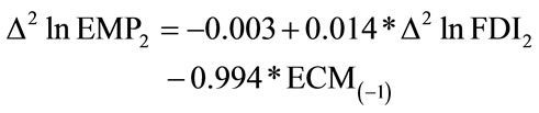 (4.7)
(4.7)
[–0.307] [0.432] [–4.411]***
R2 = 0.510 DW = 1.763
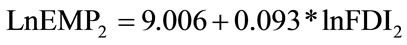
LM(1) = 2.481 LM(2) = 1.558 The result shows, in the long run, there is equilibrium relation between FDI and employment in the secondary industry, and FDI has a positive impetus on employment, with its long-run elasticity as 0.093 (3.6); while in the short term, FDI inflow of the same time period, namely t, is inimical to the growth of employment (–0.02), while FDI inflow of t – 1 period presents a positive influence on employment (0.011); however, employment of the current time period, t, is by large positively determined by the employment of the last time period, t – 1, with a coefficient as 0.987, and statistically significant so; any deviation
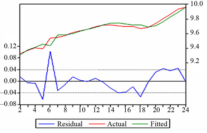
Figure 2. Actual and fitted values and residuals.
from the equilibrium will be effectively corrected at a coefficient of 0.994 (4.7), and also statistically signifycant (p-value [–4.411]***).
We tend to conclude that in the long term employment growth responds positively to the FDI inflow; in the short run, FDI inflow poses statistically limited impact on the growth of employment, and it tends to decrease the employment in the current period, whilst increase employment of the next period; moreover, employment growth is largely determined by its own; any short-run deviation from long-run equilibrium would be effectively corrected.
4.2. Tertiary Industry
The long term relations between lnEMP3 and lnFDI3 is showed as (3.8), the DW value “0.3930” shows that there is series correlation; and lagged dependent variable shall be introduced to eliminate influence of series correlation:
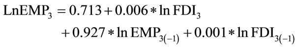
[1.796]*[0.445] [19.988]***[0.08] (4.8)
R2 = 0.992 DW = 2.323 LM(1) = 0.663 LM(2) = 0.320 LM(3) = 0.214 Judging from DW value and the LM tests for lag length of 1, 2 and 3, there is no series correlation for Equation (4.8). Residual series  is estimated as follow to further explore its stationarity:
 (4.9)
(4.9)
[–5.6481]***
R2 = 0.603 DW = 2.044 LM (1) = 0.257 LM (2) = 0.135 T-statistics and LM test for one and two lag lengths present robust evidence that Equation (4.8) is stationary; to further explore its fitness, actual and fitted values and residuals are graphed in Figure 3.
The virtual coincidence between the actual and fitted

Figure 3. Actual and fitted values and residuals.
values is quite remarkable in (4.8). The early short growth phase, the following slight fluctuation and the steadily growth phase are almost perfectly tracked by the estimated equation. The residual series is I(0) under the ADF test, with test statistics carrying a probability of nearly zero.
First-order error correction model is created as follow:

[3.437]*** [–1.727]* [–0.909] (4.10)
R2 = 0.317 DW = 1.758
LM(1) = 2.553 LM(2) = 1.657 The co-integration estimation allows us to further identify the long-run and short run relations between, say, FDI and employment. In the long run, employment responds positively to the changes in FDI, with a coefficient as 0.1878 and statistically significant so.
In the short run, impact of FDI is not statistically significant, but does pose positive impact on employment of the same time period (4.8). FDI might not impact shortterm employment growth significantly, and employment growth is its main attractor (0.927) of its last time period. FDI inflows to the tertiary industry seem to be driven by the inexorable growth of the employment.
As for the changes in the short-run disequilibrium (4. 10), employment responds negatively to the changes in FDI, though the influence might be quite slight with a coefficient as –0.008; with the statistically insignificant coefficient of ECM, deviation from long-run equilibrium would be corrected at somewhat lower speed compared with secondary industry.
Findings in the Granger Causality test provide a feasible explanation for the statistically sort of insignificant impact of FDI on employment. There is bidirectional linkage between LnEMP3 and LnFDI3, and p-value of Granger causality from lnEMP3 to lnFDI3 is even more conspicuous than that from the inverse direction, which is generally consistent with (4.8), where employment growth is the main attractor for FDI inflow.
Hence we can conclude that in the long run, FDI possesses a positive impetus on the growth of employment; whilst in the short run, FDI presents a limited influence on employment, and employment growth is by large generated by its own.
5. Conclusions
In this paper the author has explored the fundamental relations between FDI and employment of three strata industries in china over the past twenty-four years. Conclusions can be extracted as follows.
1) In the long run, growth of FDI would promote employment of the second and tertiary industry, especially the tertiary industry, where there is bidirectional linkage between FDI and employment. This positive role FDI plays in the long term would be conductive to the transition of labor force from primary to secondary industry and secondary to tertiary industry, therefore enhance the upgrade of China’s industry structure and promote the optimization of employment structure.
2) Short-term limited, even negative, impact of FDI and the main attractor role of employment indicate the increase of employment would not only cause employment growth in the next time period, but attract more FDI into the industry, and this is particularly the case for tertiary industry.
3) The policy prescription derived therefore would be directing FDI inflow to China from agricultural sectors to industrial and particularly service sectors, where FDI poses much more important impact on employment promotion and enjoys far greater role in the optimization of employment structure.
REFERENCES
- UNCTAD, “Foreign Direct Investment and the Challenge of Development,” World Investment Report, UN, New York, 2005.
- Y. P. Niu, “FDI and Quantities of Employment in China,” Economics Perspectives, Vol. 4, No. 11, 2001, pp. 29-32.
- S. Sumon and S. Klaus, “Determinants of Employment Growth at MNEs,” Working Paper, William Davidson Institute, Ann Arbor, 2004.
- J. L. Ford, S. Sen and H. X. Wei, “FDI and Economic Development in China 1970-2006: A Co-Integration Study,” Discussion Paper, University of Birmingham, Birmingham, 2010.
- F. Cai and D. W. Wang, “FDI and Employment—A Human Capital Framework,” Collected Essays on Finance and Economics, Vol. 1, No. 1, 2004, pp. 1-14.
- E. Z. Zhang and Z. C. Ren, “FDI and the Evolution of China’s Employment Structure,” Economics Theory and Management, Vol. 2, No. 52005, pp. 1-7.
- T. L. Zhao, “Comparison between Industrial Classification in Chinese National Accounts and International Standard Industrial Classification for All Economic Activities (ISIC),” 8th OECD—NBS Workshop on National Accounts, Paris, 6-10 December 2004.
- R. F. Engle and C. W. J. Granger, “Co-Integration and Error Correction: Representation, Estimation and Testing,” Econometrica, Vol. 55, No. 2, 1987, pp. 251-276. doi:10.2307/1913236
- D. A. Dickey and W. A. Fuller, “Distributions of the Estimators for Autore-Gressive Time Series with a Unit Root,” Journal of American Statistical Association, Vol. 74, No. 366, 1979, pp. 427-431. doi:10.2307/2286348
- D. A. Dickey and W. A. Fuller, “Likelihood Ratio Statistics for Autoregressive Time Series with a Unit Root,” Econometrica, Vol. 49, No. 4, 1981, pp. 1057-1072. doi:10.2307/1912517
- R. Davidson and J. G. MacKinnon, “Artificial Regressions and C ([alpha]) Tests,” Economics Letters, Vol. 35, No. 2, 1991, pp. 149-153. doi:10.1016/0165-1765(91)90162-E
- J. G. MacKinnon, “Critical Values for Cointegration Tests,” In: R. F. Engle and C. W. J. Granger, Eds., LongRun Economic Relationships, Oxford University Press, Oxford, 1991, pp. 267-276.
- C. W. J. Granger, “Investigating Causal Relations by Econometric Models and Cross-spectral Methods,” Econometrica, Vol. 37, No. 3, 1969, pp. 424-438. doi:10.2307/1912791
- C. Granger, “Some Recent Developments in a Concept of Causality,” Journal of Econometrics, Vol. 39, No. 1-2, 1988, pp. 199-211. doi:10.1016/0304-4076(88)90045-0
- R. F. Engle and C. W. J. Granger, “Co-Integration and Error Correction: Representation, Estimation and Testing,” Econometrica, Vol. 55, No. 2, 1987, pp. 251-276. doi:10.2307/1913236
- J. E. H. Davidson, D. F. Hendry, F. Srba and S. Yeo, “Econometric Modelling of the Aggregate Time-Series Relationship between Cosumers’ Expenditure and Income in the United Kingdom,” The Economic Journal, Vol. 88, No. 352, 1978, pp. 661-692. doi:10.2307/2231972
NOTES
1It is the revised version based on GB/T4754-1994; and in GB/T4754- 2002 version, service activities for agriculture, forestry, animal husbandry and fishing are shifted to primary industry, as compared with the version of 1994 in which they are in the tertiary industry.
2Traffic, transport, storage and post; Information transfer, computer services and software; Wholesale and retail trade; Accommodation and Restaurants; Finance; Real estate; Tenancy and business services; Scientific research, technical service and geologic perambulation; management of water conservancy, environment and public establishment; Resident services and other services; education; sanitation, social security and social welfare; culture, sports and entertainment; public management and social organization.
3Response Surface Study, MacKinnon 1991.
4Unit root test for residuals of second-order nonstationary time series follows the equation as: Δ2yt = α + γΔyt–1 + ∑δjΔ2yt–j + εt,(j = 1,···, p), (H0: γ = 0, H1: γ < 0), critical value is same with first-order, which is MacKinnon Engel-Granger co-integration critical values.