Communications and Network
Vol.5 No.4(2013), Article ID:39573,8 pages DOI:10.4236/cn.2013.54036
Dynamic Relay Selection Method for Distributed MIMO Relay System
Division of Physics Electrical and Computer Engineering, Graduate School of Engineering, Yokohama National University, Yokohama, Japan
Email: phamthanhhiep@gmail.com
Copyright © 2013 Pham Thanh Hiep. This is an open access article distributed under the Creative Commons Attribution License, which permits unrestricted use, distribution, and reproduction in any medium, provided the original work is properly cited.
Received August 14, 2013; revised September 5, 2013; accepted September 10, 2013
Keywords: Distributed MIMO Relay System; Optimizing Distance; Optimization Antenna Element; Upper Bound of Channel Capacity; Dynamic Relay Selection
ABSTRACT
The research on distributed MIMO relay system has been attracting much attention. In this paper, a decode-and-forward scheme distributed MIMO relay system is examined. For upper bound of channel capacity, the distance between transceivers is optimized when the propagation loss is brought close to actuality. Additionally, the number of relay is optimized whether total antenna element is fixed or not. When the number of relay is assumed to be infinite, the dynamic relay selection method based on the transmission rate is proposed. We represent that with the proposed method, the transmit power and the number of relays are saving.
1. Introduction
In the future, it is believed that the MIMO service area will become fashionable. Thus, an expansion of a service area to an isolated area is requested. Based on this idea, the authors have proposed a general idea of a MIMO relay system that can maintain the ability of highspeed and/or high-reliability data transmission [1-5]. A MIMO relay system can relay radio signals from a MIMO service area to an isolated area. In general, when a MIMO relay system has only one relay, the whole channel in the MIMO relay system is equivalent to a MIMO multi-keyhole environment. In a multi-keyhole environment, the probability density functions (PDFs) of singular values of channel response matrix or eigenvalues of correlation matrix are important from a viewpoint of system designing such as transmission characteristic meaning channel capacity and bit error rate analysis. When the number of antennas at relay is less than that at the transmitter and the receiver, the channel capacity of MIMO relay system is smaller than the one of original MIMO system. In addition, when the number of antennas at each relay is equivalent to the one of the transmitter and the receiver, a MIMO relay system can provide the same averaged channel capacity as an original MIMO system. However in case the number of antennas of each relay is larger than that of the transmit and the receive, the channel capacity of a MIMO relay system cannot exceed that of original MIMO system [6].
Therefore, in order to obtain the high channel capacity, antennas are distributed to many relays (RS), and those relays are arranged in series from the transmitter to the receiver. This system is called a distributed MIMO relay system (DMRS). In DMRS, when the distance between the transmitter and the final receiver (named total distance) is fixed, the distance between transmitter and the first relay, relay and relay, the final relay and the receiver (called between transceivers for short) is shortened, consequently the signal-to-noise ratio (SNR) as well as the channel capacity is increased. The upper bound of channel capacity is achieved by optimizing the distance between transceivers. The analysis amplify-and-forward scheme DMRS was represented in [7]. In this paper, we consider decode-and-forward scheme DMRS when the propagation loss is brought close to actuality. In such environment, the upper bound of channel capacity is achieved by optimizing the distance between transceivers in the case of fixing total transmit power and total distance. The optimum number of antennas of each relay in the sense of the largest channel capacity is obtained when the total antennas is fixed. Furthermore, when the number of relays is assumed to be infinite, the performance of system is analyzed and the dynamic relay selection method for conservation of transmit power is proposed.
The rest of paper is organized as follows. The system model of DMRS is explained in Section 2. Section 3 analyzes the system which has interference. The specific access control on Mac layer is described in Section 4. The end-to-end channel capacity of the outdated system is analyzed in Section 5. Finally, Section 6 concludes the paper.
2. Distributed MIMO Relay System
2.1. System Model
In this section, we represent obviously the DMRS with  relays intervened. The structure of system is shown in Figure 1. Here Tx, Rx and
  is the transmitter, the final receiver and the
  relay, respectively.
  denotes the number of antennas and
  denotes the distance between each transceivers. In such system, the signal is transmitted from the Tx to the
 . After that the signal is processed and forwarded to the
 . Similarly, the signal is transmitted over and over until to the final receiver.
The system parameters of each transceiver such as transceiver signal, transmit power matrix, noise vector, amplification factor of every relays are summarized in Table 1.
As expressed in Figure 2, let the channel capacity and the path loss between each transceivers is  and
and , respectively. C denotes the channel capacity of system. Let
  denotes a channel matrix between each transceivers and
  is a matrix with in-

Figure 1. System model of distributed MIMO relay system.
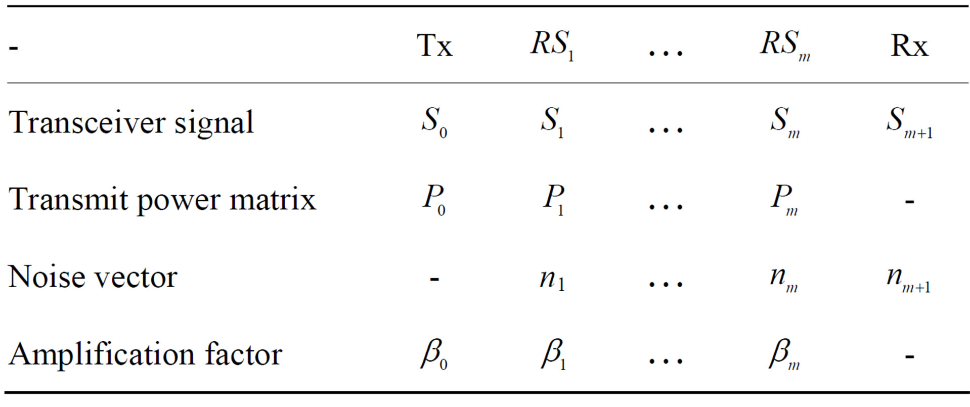
Table 1. System parameters of each transceiver.
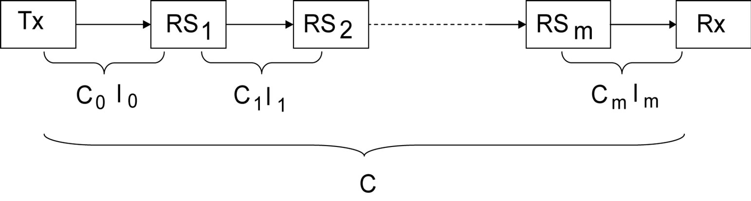
Figure 2. Channel capacity of DF scheme distributed MIMO relay system.
dependent and identically distributed (i.i.d.), zero mean, unit variance, circularly symmetric complex Gaussian entries.
Since there are several schemes for interference cancellation by using array antenna such as linear (ZF) and nonlinear (SIC/DPC) algorithm, we assume that the interference signal from other transmitters can be ignored without loss of generality. Therefore, when the signal  is transmitted from
 , the received signal at the next relay is expressed as
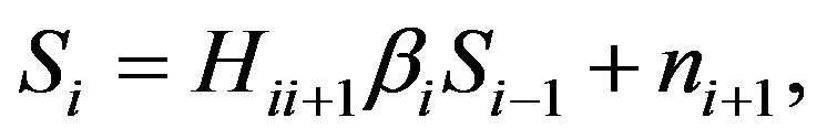 (1)
(1)
where  denotes an amplification factor of
 . In this paper, since the decode-and-forward method is applied, the amplification factor is expressed as
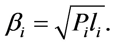 (2)
(2)
Furthermore, the channel capacity is as follows,
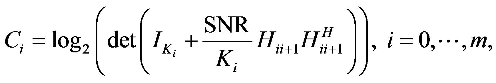 (3)
(3)
where  is
is  unit matrix. However, as described in Sect. 1, if the number of antennas at least one relay is smaller than that of other relays, this relay will be the bottleneck of system. Therefore the channel capacity of system will be decreased. In order to obtain high propagation characteristic, we assume the number of antennas at each relay to be the same. In addition,
  can be assumed to be an unit matrix. Consequently, the SNR can be examined instead of channel capacity. Since the channel capacity
  is independent of other ones, the channel capacity of the system is expressed as
 (4)
(4)
Thus the upper bound of channel capacity of system is achieved when the channel capacity of every receivers meaning the SNR of every receivers is equivalent. Therefore, it is necessary to optimize the distance between each transceivers in order to obtain the upper bound of channel capacity of system.
2.2. Propagation Loss
We assume that the transmit power of each relay is kept the same regardless of the total transmit power of relays as well as the number of relay is fixed or not. Therefore, the SNR is proportional to a propagation loss. Since the propagation channel is not always a free-space propagation, so it is necessary to consider being attenuated by the reflection, scattering, and so on. The propagation loss in this case, namely a multi-path propagation environment is expressed as
 (5)
(5)
Here,  and
and  denote the wavelength and the reflection times, respectively. The reflection loss
  is defined as an amount of the attenuation by only one reflection. However, the propagation loss of multi-path propagation environment is complex. In order to analyze the distributed MIMO relay system, the propagation loss is simplified by using only maximum receiver SNR path as
 (6)
(6)
For validating the simplified loss, the parameter summarized in Table 2 is used to compare the original path loss to the simplified path loss.
Figure 3 shows the received power of the original propagation loss and the simplified loss. The original path loss is approximated by the simplified path loss with the ratio of 1.16. Thus, the simplified path loss can be used instead of original path loss to analyze the DMRS.

Table 2. Parameters for validation of the simplified loss.

Figure 3. The received power of original path loss and the simplified path loss.
2.3. Propagation Environment
We consider the DMRS for several wireless networks such as 1) Extension a MIMO service area from a base station in center of city to a receiver terminal in country side, 2) Transmission a health information from monitors implanted in body to a receiver of the outside, 3) Transmission information from terminals in isolated area to the near base station. For all of these scenarios, the environment around the Tx has a lot of transmission obstacle, consequently the signal reflects many times before arriving the next relay. The number of reflections is decreased when the signal goes away from the Tx. In addition, the number of reflections is proportional to distance between each transceiver. Thus, we define the number of reflections when the signal is transmitted from the  to
to  as follows.
 (7)
(7)
where  denotes the distance between the Tx and the
 . The propagation environment coefficient
  is defined as the average line of sight (LOS) distance from the Tx to the
 . Figure 4 shows the average number of reflections between each transceivers when the distance between each transceivers is changed, i.e. 250 m, 500 m, and the propagation environment coefficient
  is 500 m.
As the result shown in Figure 4, the shorter the distance between each transceivers is and/or the farther from the Tx a relay is, the smaller the average number of reflections becomes. It means that the Equation (7) can describes correctly the propagation environment that we consider to apply this research to.
3. Upper Bound of Channel Capacity When Total Transmit Power and Distance Are Fixed
3.1. Optimizing Distance
We assume that the total transmit power  is fixed in spite of the change in the number of relays and the number of antennas at each relay. In order to simplify the composition of relay, the total transmit powers is equally divided into each relay. Moreover, the transmit power of each relay is equally divided into each antenna. Therefore, let
  denote the transmit power of one antenna, every transmit power matrix is expressed as
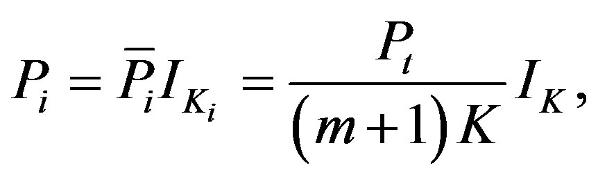 (8)
(8)
where  is the number of antennas of a relay. In order to obtain the upper bound of channel capacity of system, all of SNR are necessary to be equal.

Figure 4. Average number of reflections.
 (9)
(9)
where
 (10)
(10)
and  denotes the covariance of noise vector in each relay and the final receiver. By solving (9), the optimized distances are obtained. Figure 5 shows the optimized distance of each relay in case the number of relays is 5. The parameter is summarized in Table 3. As shown in Figure 5, the optimized distance between each transceivers is increased when the relay goes far from the Tx. The reason can be explained that when the relay is far from the Tx, the average number of reflections become smaller, therefore, in the same channel capacity, the signal can be transmitted farther.
3.2. Upper Bound of Channel Capacity
In this section, we examine the upper bound of channel capacity in some different system models. Firstly, the propagation environment is changed. Figure 6 shows the upper bound of channel capacity when D is 500 m and 1500 m. Since the number of reflections is decreased when D is increased, the channel capacity when  is 1500 m, is larger than the one of
  being 500 m. When the number of relay is increased, the distance between each transceivers is shorten, therefore the channel capacity is increased.
Then, we examine the upper bound of channel capacity when total transmit powers is changed, i.e., 100 mW, 300 mW, 500 mW. As the channel capacity shown in Figure 7, the bigger the transmit power is, the higher the upper bound of channel capacity becomes. Therefore, in order to obtain the same channel capacity, the large number of relay is requested if the total transmit power is small.
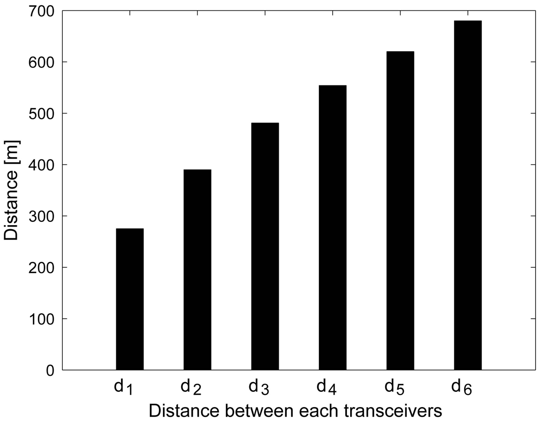
Figure 5. The optimized distance between each transceivers in a sense of upper bound of channel capacity.
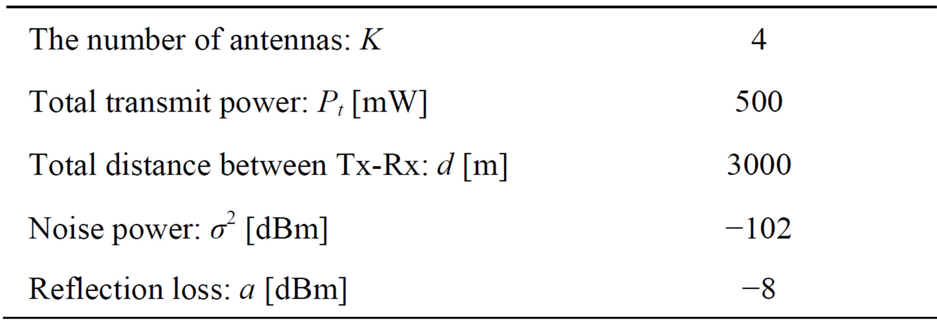
Table 3. Numerical parameters.

Figure 6. The upper bound of channel capacity when the propagation environment changes.
3.3. Optimizing the Number of Antennas When Total Number of Antennas Is Fixed
Up to now, we have analyzed the performance of DMRS where the number of relays as well as the number of antennas are assumed to be infinite. However from the viewpoint of the cost and the place, it is necessary to analyze the performance of system when the number of antennas is finite. As described in previous section, for high channel capacity, a lot of relay is demanded. However, for MIMO propagation, the number of antennas at each relay plays an important rule as expressed in (3).
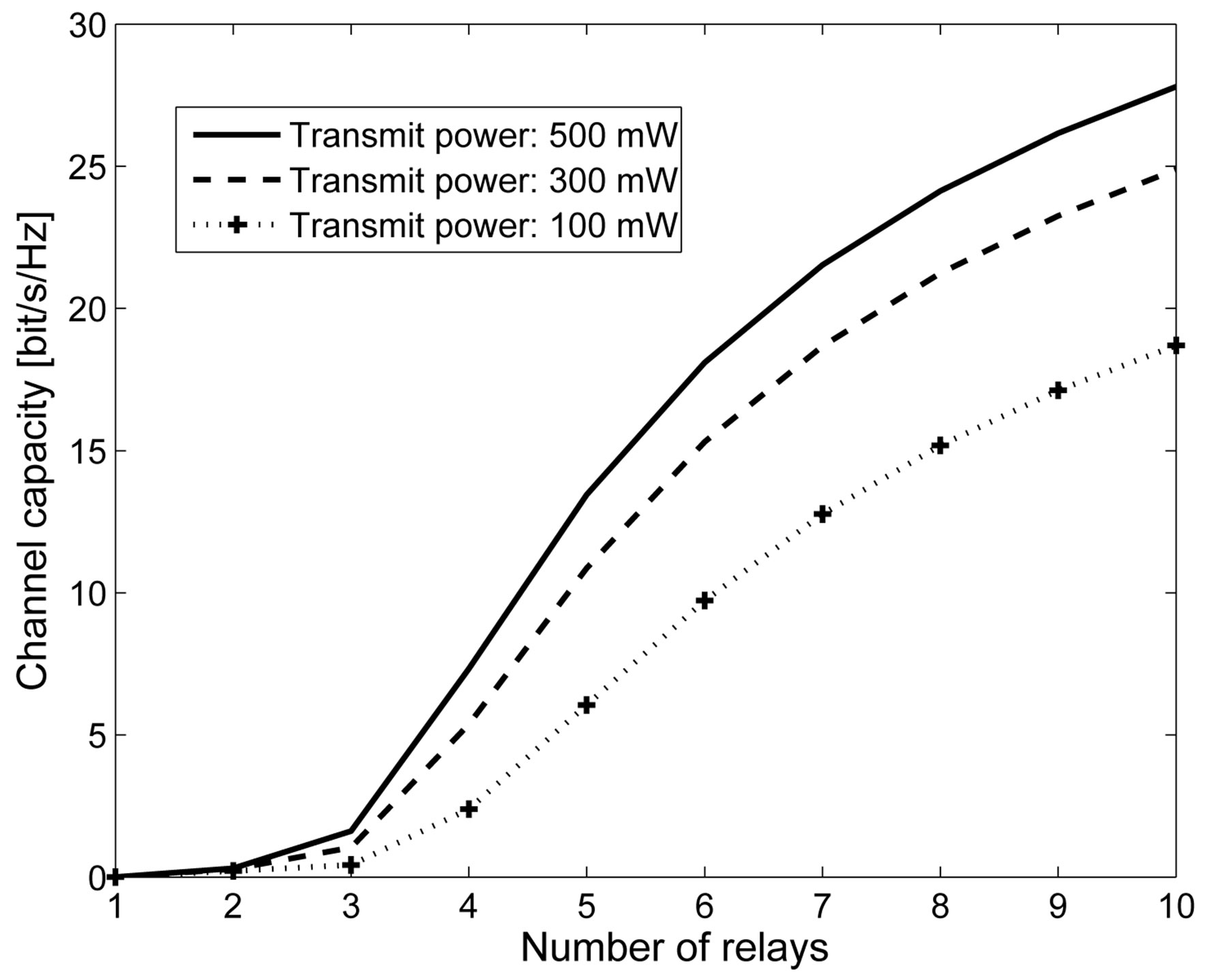
Figure 7. The upper bound of channel capacity when the total transmit power changes.
Consequently, the relation between the number of relays and the number of antennas at each relay needs to be considered. Let us assume that the total antennas is T. Since the number of antennas at every relay is assumed to be equal, the number of antennas at each relay becomes
 (11)
(11)
where  denotes the number of relays. In fact, the number of antennas is an integral number, however, in order to analyze the performance of system easily, we assume the number of antennas is a positive number. The channel capacity of each transceivers is changed as
 (12)
(12)
The parameter is summarized in Table 3. The upper bound of channel capacity is shown in Figures 8 and 9.
As shown in Figure 8, there is an optimal number of relays, meaning the optimal number of antennas at each relay in the sense of the largest channel capacity. If the number of relays is smaller than the optimal number, the distance between each transceiver is increased. As a result, the channel capacity is decreased. On the other hand, if the number of relay is higher than the optimal number, the distance between each transceiver is shortened, consequently the SNR is increased. However the number of antennas at each relay is decreased, therefore the channel capacity is decreased. Furthermore, the optimal number of antennas is changed when the propagation environment or the total transmit power is changed (Figure 9). In the same propagation environment and total transmit power, the optimal number of relays is almost the same though total number of antennas is changed.

Figure 8. The upper bound of channel capacity when the total antennas is fixed, i.e 10, 20, and 40.

Figure 9. The upper bound of channel capacity in different channel models when total antennas is 10.
4. Maximum of Total Distance
Up to now, the upper bound of channel capacity was analyzed when the total distance is fixed. However, in case of expansion service area, the transmit power of relay as well as the transmission rate are fixed. Therefore, the analysis of system when the transmission rate is fixed, is necessary.
4.1. Maximum of Total Distance
At first, we analyze the maximum of total distance when the transmit power of each relay and the number of relays are fixed. In this case, the maximum of distance between each transceivers  must satisfies the next condition.
 (13)
(13)
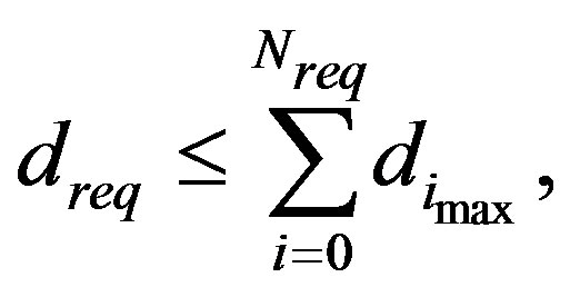
here P and Creq denote the transmit power of each transmitter and the requested channel capacity, respectively. Let the number of relays is M, the maximum of total distance for each requested channel capacity becomes
 (14)
(14)
The parameter is summarized in Table 4. The maximum of total distance in case the number of relay is 5 and 10, is shown in Figure 10.
For the same requested channel capacity, the smaller the number of relay is, the shorter the maximum of total distance becomes. In addition, the maximum of total distance is rapidly decreased when the requested channel capacity is increased.
4.2. The Necessary Number of Relays
In case the total distance and the channel capacity are fixed, the analysis of number of relays is requested. The necessary relay number  must to satisfies next equation while the maximum of distance between each transceivers follows (13).
 (15)
(15)
here  denotes the distance from the Tx to the Rx.
The parameter summarized in Table 4 is used and the distance from the Tx and the Rx is fixed at 3000 m, the necessary number of relays is shown in Figure 11. When the channel capacity is increased, the necessary number

Table 4. Parameters for maximum of total distance.
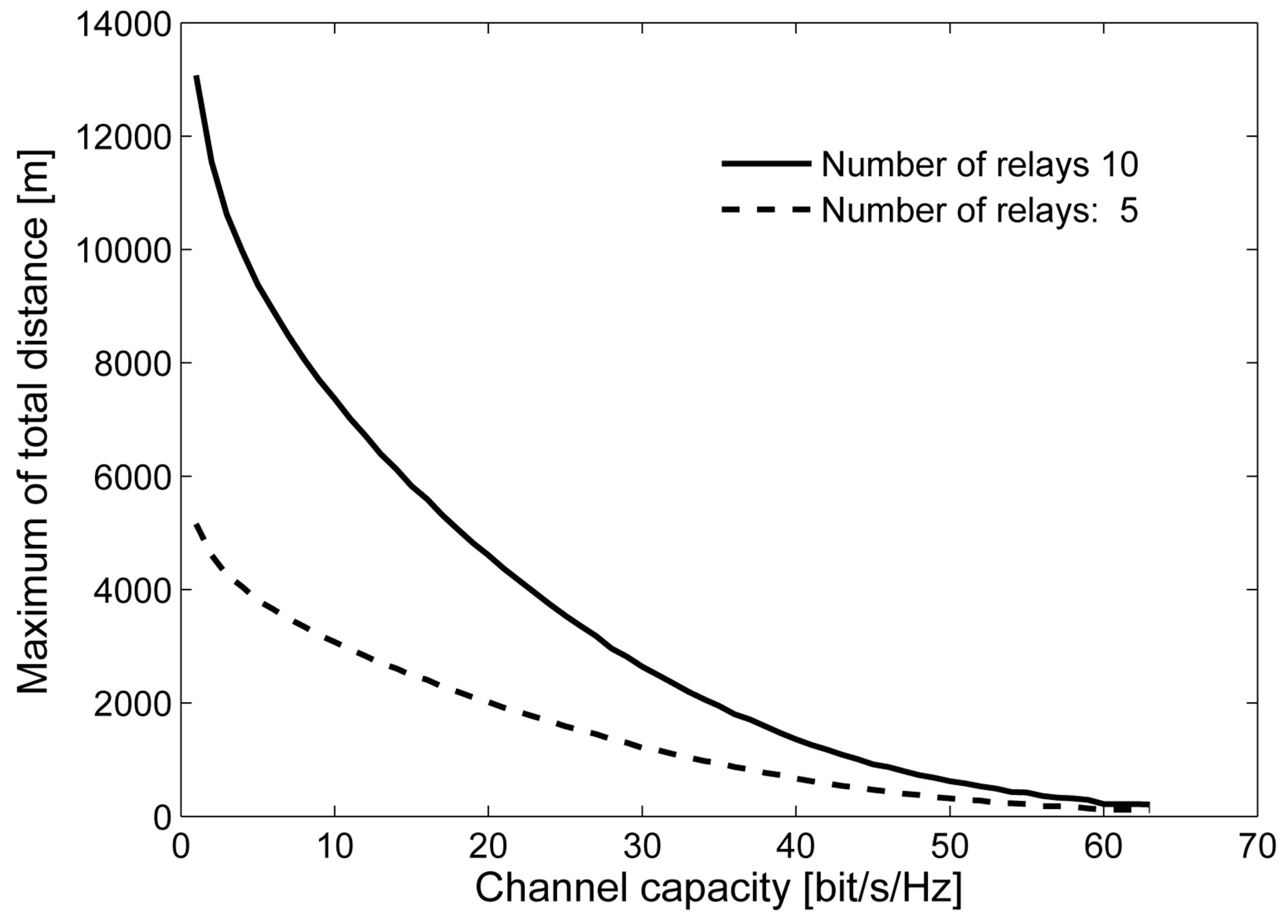
Figure 10. The maximum of total distance for each requested channel capacity.

Figure 11. The necessary number of relays for each channel capacity.
of relays is considerably increased. However, each number of relays can cover a range of several channel capacities.
5. Dynamic Relay Selection Method for Conservation of Transmit Power
5.1. Dynamic Relay Selection Method
The upper bound of channel capacity of peer-to-peer system was analyzed in previous sections. However, in fact, imultiple terminals may access to the relay system via the nearest relay (Figure 12). Therefore, each relay receives the signal from not only the previous relay, but also from terminals around itself and sends the total data to the next relay or the Rx.
Let  denotes the transmission data of
  and
and  denote the total transmission data of the terminals around
 . Therefore, the transmission data of
  must be
 . In this section, we assume that there are many relays that be arranged from the Tx to the Rx and each relay knows the distance from itself to the others as well as the propagation environment. Each relay can selects the next relay to transmit the signal. The next relay is the one that the current relay can transmit total data to. For saving the relay and the transmit power, if there are many relays that the current relay can transmit total data to, the farthest relay is selected. In short, the distance from the current relay to the next relay must satisfies that
 (16)
(16)
This selection method is called dynamic relay selection method.
5.2. Conservation of Transmit Power
The dynamic relay selection method is compared to the
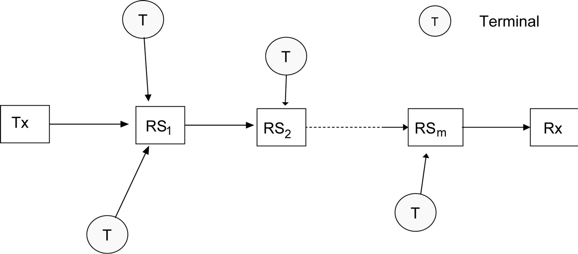
Figure 12. System model of dynamic relay selection method.
optimizing distance method that described in Sec. 3.1. In case of optimizing distance method, the total transmit power is fixed, and the channel capacity between each transceivers is the same. On the other hand, in case of dynamic relay selection method, the transmit power of each relay is fixed, however the total transmit power is infinite, and the channel capacity between each transceivers is different. We assume that the data that received at the Rx in an unit time is the same in both methods, however the transmission data of the Tx and terminals is random value. The parameter is summarized in Table 3, and the propagation environment coefficient D is assumed to be 1500 m. The DMRS transmits the signal with channel capacity that is expressed in Figure 6. Therefore the transmit power and the number of relays of optimizing distance method is as expressed in Figure 6. The transmit power of each relay in case of dynamic relay selection method P is assumed to be 100 mW and 50 mW. Figures 13 and 14 show the necessary transmit power and the number of relay, respectively.
When the channel capacity is low, the transmit power of dynamic relay selection method is considerably smaller than that of optimizing distance method. However when the channel capacity is increased, the transmit power of dynamic relay selection method is increased and be higher than the one of optimizing distance method as described in Figure 13. On the contrary, when the channel capacity is low, the necessary relay number of dynamic selection method is larger than that of optimizing distance method. When the channel capacity is increased, the relay number of dynamic relay selection method is increased, however it becomes smaller than the one of optimizing distance method (Figure 14).
On the other hand, In case P = 100 mW of dynamic relay selection method, when the channel capacity is within 17 and 28 bit/s/Hz, both the necessary transmit power and the number of relays are lower than that of optimizing distance method. Similarly, in case P = 50 mW of dynamic relay selection method, when the channel capacity is over 25 bit/s/Hz, both the necessary transmit power and the number of relays are lower than that of optimizing distance method.
As two examples mentioned before, by adjusting the
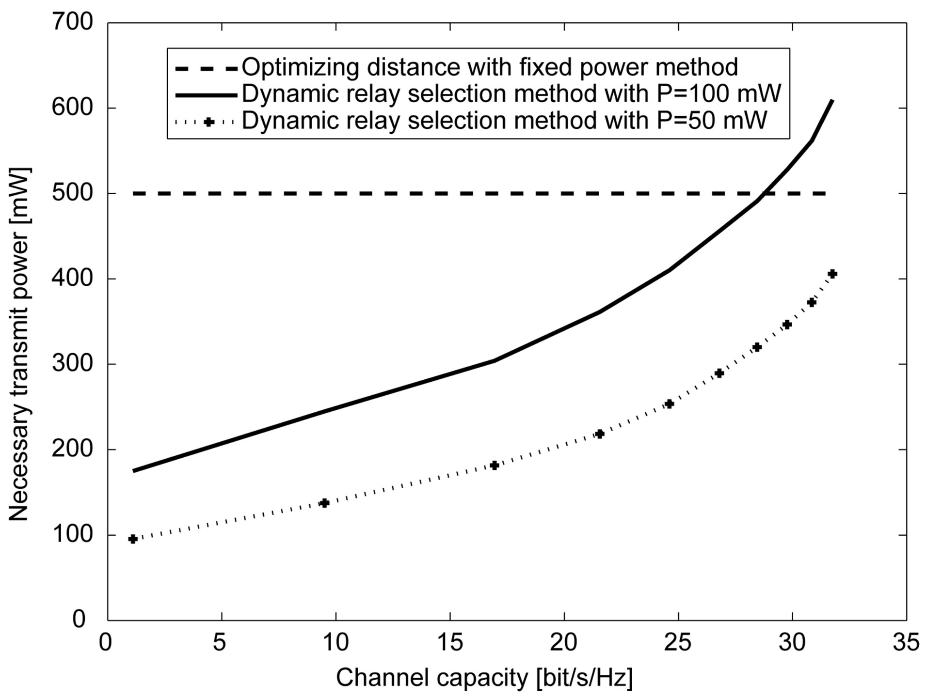
Figure 13. The necessary transmit power in both methods, P = 50 mW and 100 mW.

Figure 14. The necessary number of relays in both methods, P = 50 mW and 100 mW.
transmit power of each relay, with lower total transmit power and the smaller number of relays, the dynamic relay selection method can transmit the same channel capacity as the optimizing distance method.
6. Conclusions
In this paper, the performance of a DMRS with decodeand-forward method was examined. For upper bound of channel capacity of the system, the position of all relays meaning the distance between transceivers was optimized in case of fixing transmit power, total distance and total antenna elements. When total antenna element is fixed, there is the optimum number of antennas in the sense of the largest channel capacity, the optimum of antenna element number is changed by changing in condition of transmission. The dynamic relay selection method was proposed for conservation of transmit power and the number of relays.
The pear-to-pear(P2P) transmission method and the multiple-users to one-user (M2P) transmission method have been considered in this paper. In the future, not only the P2P and M2P transmission method, but also multipleuser to multiple-user (M2M) transmission method will be considered. In addition, the network coding will be applied to this research.
REFERENCES
- D. Chizhik, G. J. Foschini, M. J. Gans and R. A. Valenzuela, “Keyholes, Correlations, and Capacities of Multielement Transmit and Receive Antennas,” IEEE Transactions on Wireless Communications, Vol. 1, No. 2, 2002, pp. 361-368. http://dx.doi.org/10.1109/7693.994830
- D. Gesbert, H. Bolcskei, D. A. Gore and A. J. Paulraj, “MIMO Wireless Channel: Capacity and Performance Prediction,” Proceedings of Global Telecommunications Conference, GLOBECOM'00, San Francisco, 27 November-1 December 2000, pp. 1083-1088.
- B. Wang, J. Zhang and A. Host-Madsen, “On the Capacity of MIMO Relay Channel,” IEEE Transactions on Information Theory, Vol. 51, No. 1, 2005, pp. 29-43. http://dx.doi.org/10.1109/TIT.2004.839487
- S. M. Alamouti, “A Simple Transmit Technique for Wireless Communications,” IEEE Journal on Selected Areas in Communications, Vol. 16, No. 8, 1998, pp.1451-1458. http://dx.doi.org/10.1109/49.730453
- V. Tarokh, N. Seshadri and A. R. Calderbank, “SpaceTime Codes for High Data Rate Wireless Communication: Performance Critrion and Code Constraction,” IEEE Transactions on Information Theory, Vol. 44, No. 2, 1998, pp.744-765. http://dx.doi.org/10.1109/18.661517
- M. Tsuruta, T. Taniguchi and Y. Karazawa, “On Statistical Distribution of Eigenvalues of Channel Correlation Matrix in MIMO Multi-Keyhole Environment,” The IEICE Transaction on Communications, Vol. E90-B, No. 9, 2007, pp. 2352-2359.
- P. T. Hiep, C. Sugimoto and R. Kohno, “MAC-PHY Cross-Layer for High Channel Capacity of Multiple-Hop MIMO Relay System?” Communications and Network, Vol. 4, No. 2, 2012, pp. 129-138. http://dx.doi.org/10.4236/cn.2012.42017