World Journal of Mechanics
Vol.3 No.6(2013), Article ID:36845,15 pages DOI:10.4236/wjm.2013.36029
Bifurcation and Chaos of Gear Pair System Supported by Long Journal Bearings Based on Turbulent Flow Effect and Nonlinear Suspension Effect
Department of Mechanical and Automation Engineering, I-Shou University, Kaohsiung City, Chinese Taipei
Email: cwchangjian@mail.isu.edu.tw
Copyright © 2013 Cai-Wan Chang-Jian. This is an open access article distributed under the Creative Commons Attribution License, which permits unrestricted use, distribution, and reproduction in any medium, provided the original work is properly cited.
Received July 17, 2013; revised August 15, 2013; accepted September 2, 2013
Keywords: Gear Pair; Long Journal Bearing; Nonlinear Suspension; Turbulent Flow
ABSTRACT
A systematic analysis of the dynamic behavior of a gear-bearing system with nonlinear suspension, turbulent flow effect, long journal bearing approximation, nonlinear oil-film force and nonlinear gear mesh force is performed in the present study. The dynamic orbits of the system are observed by bifurcation diagrams plotted using the dimensionless unbalance coefficient and the dimensionless rotational speed ratio as control parameters. The onset of chaotic motion is identified from the phase diagrams, power spectra, Poincaré maps, Lyapunov exponents and fractal dimension of the gearbearing system. The numerical results reveal that the system exhibits a diverse range of periodic, sub-harmonic, quasiperiodic and chaotic behaviors. The results presented in this study provide some useful insights into the design and development of a gear-bearing system for rotating machinery that operates in highly rotational speed and highly nonlinear regimes.
1. Introduction
We all know that dynamic analyses of turbo-machineries are complicated but significant. Nevertheless, most studies focused on studying dynamics of single mechanical component of machineries e.g., rotors, bearings, gears or cams individually. Actually, individual dynamic response may influence one another of these mechanical components especially in studying nonlinear dynamic behaviors and their behaviors may couple together. Thus multimechanical components should be modeled and analyzed together, and combined nonlinear effects occurring in mechanical components to study their real dynamic responses for the whole mechanical systems. Many studies have focused on analyzing gear dynamics or relative researches.
Vedmar and Anersson [1] presented a method to calculate dynamic gear tooth force and bearing forces and the bearing model was under elastic bearings assumption. The simulation results of elastic model were somewhat different compared with stiff one. The gear mesh model using with constant was studied by a lot of people, such as Kahraman and Singh [2], Lin, et al. [3], Yoon and Rao [4], and Ichimaru and Hirano [5]. Amabili and Fregolent
[6] introduced a method based on the measurement of the gear torsional vibrations to identify natural frequency, damping parameters and equivalent gear error of a spur gear pair model. Ozguven and Houser [7,8] performed dynamic analysis on gears with the effects of variable mesh stiffness, damping, gear errors profile modification and backlash. Cai and Hayashi [9] calculated the optimum profile modification to obtain a zero vibration of the gear pair. Umezawa et al. [10] analyzed a single DOF numerical gear pair model and compared their numerical results with experimental dynamic transmission errors. Mcfadden and Toozhy [11] used the high frequency technique combined with synchronous averaging to detect the failure in rolling element bearings. Litvin, et al. [12] proposed a modified geometry of an asymmetric spur gear drive designed as a favorable shape of transmission errors of reduced magnitude and also reduced contact and bending stresses for an asymmetric spur gear drive. Guan, et al. [13] performed finite element method to simulate the geared rotor system constructed from beam and lumped mass/stiffness elements and compared the required actuation effort, control robustness and implementation cost. Giagopulos, et al. [14] presented an analysis on the nonlinear dynamics of a gear-pair system supported on rolling element bearings and used a suitable genetic algorithm to measure noise and model error. Theodossiades and Natsiavas [15] investigated dynamic responses and stability characteristics of rotordynamic systems interconnected with gear pairs and supported on oil journal bearings. They found many non-periodic dynamic behaviors. They [16] also analyzed the motor-driven gear-pair systems with backlash and found periodic and chaotic dynamics in this system.
There are also many studies analyzing performance or dynamics or relative researches of bearing systems under turbulent assumptions. Constantinescu [17] first presented a modified Reynolds equation to describe the turbulent lubrication based on the mixing length concept of Prandtl. Elrold and Ng [18] proposed an application to the combined lubricant flow of both pressure and shear flows. Hirs [19] developed a new method, based on the bulk flow concept, by relying on the relationships between wall shear stress and mean velocity relative to the wall. Hashimoto et al. [20,21] examined the effects of wear on steady state and dynamic characteristics of the theoretical and experimental methods under operating conditions including turbulence. Capone [22] predicted dynamic characteristics and stability of a journal bearing in a non-laminar lubrication regime. Kumar and Mishra [23] analyzed the stability of the rigid rotor in turbulent hydrodynamic worn journal bearing and they concluded that lower L/D ratios are more stable for worn bearings. Lahmar [24] proposed an optimized short bearing theory for nonlinear dynamic analysis of turbulent journal bearings. They also proved that the turbulent effects on the dynamic behavior of rotor-bearing systems become more significant as the journal rotational speed increases. Recently, Chang-Jian and Chen [25] studied bifurcation analysis and chaotic analysis of a flexible rotor supported by turbulent journal bearings with nonlinear suspension. It is well known that vibrations of gear pairs are significantly affected by the amplitude and phase of deviations of the tooth profile from the true involute one. Gear errors were therefore must be checked in order to avoid bad working conditions for high speed gears and precision manufacturing. Although many researches focused on the analysis of the hydrodynamic lubrication of journal bearing, most of the flow of lubricant is assumed to be the laminar flow. The high speed journal bearings lubricated with unconventional lubricants of low viscosity give rise to large film Reynolds numbers, and therefore the flow of the bearing becomes turbulent.
Although virtually all physical phenomena in the real world can be regarded as nonlinear, most of these phenomena can be simplified to a linear form given a sufficiently precise linearization technique. However, this simplification is inappropriate for high-power, high rotational speed gear systems, and its application during the design and analysis stage may result in a flawed or potentially dangerous operation. As a result, nonlinear analysis methods are generally preferred within engineering and academic circles. The current study performs a nonlinear analysis of the dynamic behavior of a gear pair system equipped with long journal bearings under turbulent effect and nonlinear suspension. The non-dimensional equation of the gear-bearing system is then solved using the Runge-Kutta method. The non-periodic behavior of this system is characterized using phase diagrams, power spectra, Poincaré maps, bifurcation diagrams, Lyapunov exponents and the fractal dimension of the system.
2. Mathematical Modeling
To be able to simulate the gear-bearing system, some assumptions are presented to simplify dynamic models. The assumptions of nonlinear suspension (hard spring effect), long journal bearing, turbulent flow effect, strongly nonlinear gear meshing force and strongly nonlinear fluid film force effect are established. Figure 1 shows the gear-baring model presented in this study, and Figure 2" target="_self"> Figure 2 presents a schematic illustration of the dynamic model considered between gear and pinion. Og and Op are the center of gravity of the gear and pinion, respectively; O1 and O2 are the geometric centers of the bearing 1 and bearing 2, respectively; Oj1 and Oj2 are the geometric centers of the journal 1 and journal 2, respectively; m1 is the mass of the bearing housing for bearing 1 and m2 is
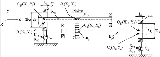
Figure 1. Schematic illustration of the gear-bearing system under nonlinear suspension.
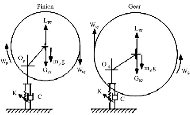
Figure 2. Model of force diagram for pinion and gear.
the mass of the bearing housing for bearing 2; mp is the mass of the pinion and mg is the mass of the gear; Kp1 and Kp2 are the stiffness coefficients of the shafts; K11, K12, K21 and K22 are the stiffness coefficients of the springs supporting the two bearing housings for bearing 1 and bearing 2; C1 and C2 are the damping coefficients of the supported structure for bearing 1 and bearing 2, respectively; K is the stiffness coefficient of the gear mesh, C is the damping coefficient of the gear mesh, e is the static transmission error and varies as a function of time. Note that (Xi, Yi) are fixed coordinates, while (ei, ji) are rotational coordinates, in which ei is the offset of the journal center and ji is the attitude angle of the rotor relative to the X-coordinate direction.
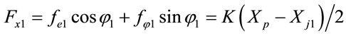
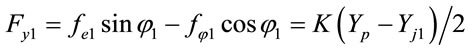
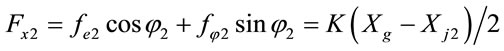
According to the principles of force equilibrium, the forces acting at the center of journal 1, i.e. Oj1(Xj1, Yj1) and center of journal 2, i.e. Oj2(Xj2, Yj2) are given by
 , (1)
, (1)
 , (2)
, (2)
 , (3)
, (3)
 , (4)
, (4)
in which fe1 and fj1 are the viscous damping forces in the radial and tangential directions for the center of journal 1, respectively, and fei2 and fj2 are the viscous damping forces in the radial and tangential directions for the center of journal 2, respectively.
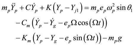
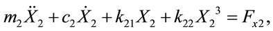
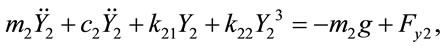
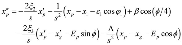
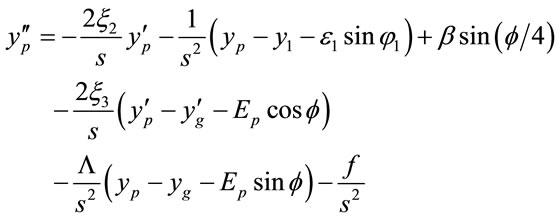
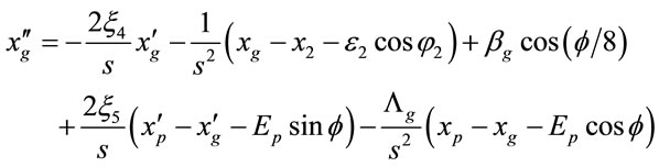
The equations of motion used to describe geometric centers of gear and pinion (Og(Xg, Yg) and Op(Xp, Yp)) can be written as
 , (5)
, (5)
 , (6)
, (6)
 , (7)
, (7)
 , (8)
, (8)
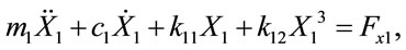
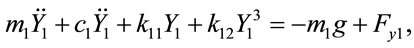
The equations of motion of the center of bearing 1 (X1, Y1) and the center of bearing 2 (X2, Y2) under the assumption of nonlinear suspension can be written as
 (9)
(9)
 (10)
(10)
 (11)
(11)
 (12)
(12)
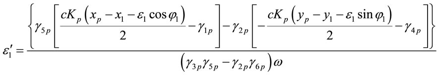
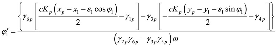
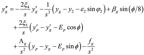
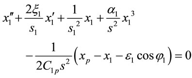
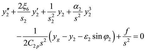
Equations (1)-(12) can be expressed as
 , (13)
 , (14)
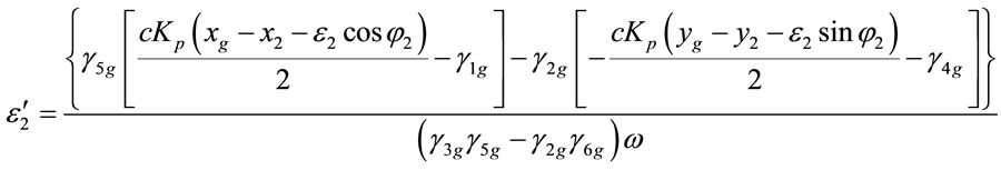 , (15)
 , (16)
 , (17)
 , (18)
 , (19)
 , (20)
 , (21)
 , (22)
 , (23)
 , (24)
Equations (13)-(24) describe a non-linear dynamic system. In the current study, the approximate solutions of these coupled non-linear differential equations are obtained using the fourth order Runge-Kutta numerical scheme.
3. Analytical Tools for Observing Nonlinear Dynamics of Gear-Bearing System
In the present study, the nonlinear dynamics of the gearbearing system shown in Figure 1 are analyzed using Poincaré maps, bifurcation diagrams, the Lyapunov exponent and the fractal dimension. The basic principles of each analytical method are reviewed in the following sub-sections.
3.1. Dynamic Trajectories and Poincaré Maps
The dynamic trajectories of the gear-bearing system provide a basic indication as to whether the system behavior is periodic or non-periodic. However, they are unable to identify the onset of chaotic motion. Accordingly, some other form of analytical method is required. In the current study, the dynamics of the gear-bearing system are analyzed using Poincaré maps derived from the Poincaré section of the gear system. A Poincaré section is a hyper-surface in the state space transverse to the flow of the system of interest. In non-autonomous systems, points on the Poincaré section represent the return points of a time series corresponding to a constant interval T, where T is the driving period of the excitation force. The projection of the Poincaré section on the  plane is referred to as the Poincaré map of the dynamic system. When the system performs quasi-periodic motion, the return points in the Poincaré map form a closed curve. For chaotic motion, the return points form a fractal structure comprising many irregularly-distributed points. Finally, for nT-periodic motion, the return points have the form of n discrete points.
3.2. Power Spectrum
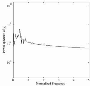
In this study, the spectrum components of the motion performed by the gear-bearing system are analyzed by using the Fast Fourier Transformation method to derive the power spectrum of the displacement of the dimensionless dynamic transmission error. In the analysis, the frequency axis of the power spectrum plot is normalized using the rotational speed, w.
3.3. Bifurcation Diagram
A bifurcation diagram summarizes the essential dynamics of a gear-train system and is therefore a useful means of observing its nonlinear dynamic response. In the present analysis, the bifurcation diagrams are generated using two different control parameters, namely the dimensionless unbalance coefficient, β, and the dimensionless rotational speed ratio, s, respectively. In each case, the bifurcation control parameter is varied with a constant step and the state variables at the end of one integration step are taken as the initial values for the next step. The corresponding variations of the  coordinates of the return points in the Poincaré map are then plotted to form the bifurcation diagram.
3.4. Lyapunov Exponent
The Lyapunov exponent of a dynamic system characterizes the rate of separation of infinitesimally close trajectories and provides a useful test for the presence of chaos. In a chaotic system, the points of nearby trajectories starting initially within a sphere of radius  form after time
  an approximately ellipsoidal distribution with semi-axes of length
 . The Lyapunov exponents of a dynamic system are defined by
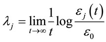 , where
  denotes the rate of divergence of the nearby trajectories. The exponents of a system are usually ordered into a Lyapunov spectrum, i.e.
 . A positive value of the maximum Lyapunov exponent
  is generally taken as an indication of chaotic motion [25].
3.5. Fractal Dimension
The presence of chaotic vibration in a system is generally detected using either the Lyapunov exponent or the fractal dimension property. The Lyapunov exponent test can be used for both dissipative systems and non-dissipative (i.e. conservative) systems, but is not easily applied to the analysis of experimental data. Conversely, the fractal dimension test can only be used for dissipative systems, but is easily applied to experimental data. In contrast to Fourier transform-based techniques and bifurcation diagrams, which provide only a general indication of the change from periodic motion to chaotic behavior, dimensional measures allow chaotic signals to be differentiated from random signals. Although many dimensional measures have been proposed, the most commonly applied measure is the correlation dimension dG defined by Grassberger and Procaccia due to its computational speed and the consistency of its results. However, before the correlation dimension of a dynamic system flow can be evaluated, it is first necessary to generate a time series of one of the system variables using a time-delayed pseudophase-plane method. Assume an original time series of  where t is the time delay (or sampling time). If the system is acted upon by an excitation force with a frequency w, the sampling time, t, is generally chosen such that it is much smaller than the driving period. The delay coordinates are then used to construct an n-dimensional vector
 where
where . The resulting vector comprises a total of
  vectors, which are then plotted in an n-dimensional embedding space. Importantly, the system flow in the reconstructed n-dimensional phase space retains the dynamic characteristics of the system in the original phase space. In other words, if the system flow has the form of a closed orbit in the original phase plane, it also forms a closed path in the n-dimensional embedding space. Similarly, if the system exhibits a chaotic behavior in the original phase plane, its path in the embedding space will also be chaotic. The characteristics of the attractor in the n-dimensional embedding space are generally tested using the function
 to determine the number of pairs (i, j) lying within a distance
  in
in , where H denotes the Heaviside step function, N represents the number of data points, and r is the radius of an n-dimensional hyper-sphere. For many attractors, this function exhibits a power law dependence on r as r ® 0, i.e.
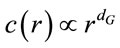 . Therefore, the correlation dimension, dGcan be determined from the slope of a plot of
  versus
 . Grassberger and Proccacia [26] showed that the correlation dimension represents the lower bound to the capacity or fractal dimension dc, and approaches its value asymptotically when the attracting set is distributed more uniformly in the embedding phase space. A set of points in the embedding space is said to be fractal if its dimension has a finite non-integer value. Otherwise, the attractor is referred to as a “strange attractor”. To establish the nature of the attractor, the embedding dimension is progressively increased, causing the slope of the characteristic curve to approach a steady state value. This value is then used to determine whether the system has a fractal structure or a strange attractor structure. If the dimension of the system flow is found to be fractal (i.e. to have a non-integer value), the system is judged to be chaotic.
In the current study, the attractors in the embedding space were constructed using a total of 60000 data points taken from the time series corresponding to the displacement of the system. Via a process of trial and error, the optimum delay time when constructing the time series was found to correspond to one third of a revolution of the system. The reconstructed attractors were placed in embedding spaces with dimensions of n = 2, 4, 6, 8, 10, 12, 14, 16, 18, and 20, respectively, yielding 10 different
 versus
  plots for each attractor. The number of data points chosen for embedding purposes (i.e. 60,000) reflects the need for a compromise between the computation time and the accuracy of the results. In accordance with Chen & Yau [27], the number of points used to estimate the intrinsic dimension of the attracting set in the current analysis is less than 42M, where M is the greatest integer value less than the fractal dimension of the attracting set.
4. Numerical Results and Discussions
The nonlinear dynamic equations presented in Equations (13) to (24) for the gear-bearing system with nonlinear suspension effects, turbulent flow effect, strongly nonlinear oil-film force and nonlinear gear mesh force were solved using the fourth order Runge-Kutta method. The time step in the iterative solution procedure was assigned a value of  and the termination criterion was specified as an error tolerance of less than 0.0001. The time series data corresponding to the first 800 revolutions of the two gears were deliberately excluded from the dynamic analysis to ensure that the analyzed data related to steady-state conditions. The sampled data were used to generate the dynamic trajectories, Poincaré maps and bifurcation diagrams of the spur gear system in order to obtain a basic understanding of its dynamic behavior. The maximum Lyapunov exponent and the fractal dimension measure were then used to identify the onset of chaotic motion. For convenience, only the data of the displacements in the vertical direction were used to generate diagrams.
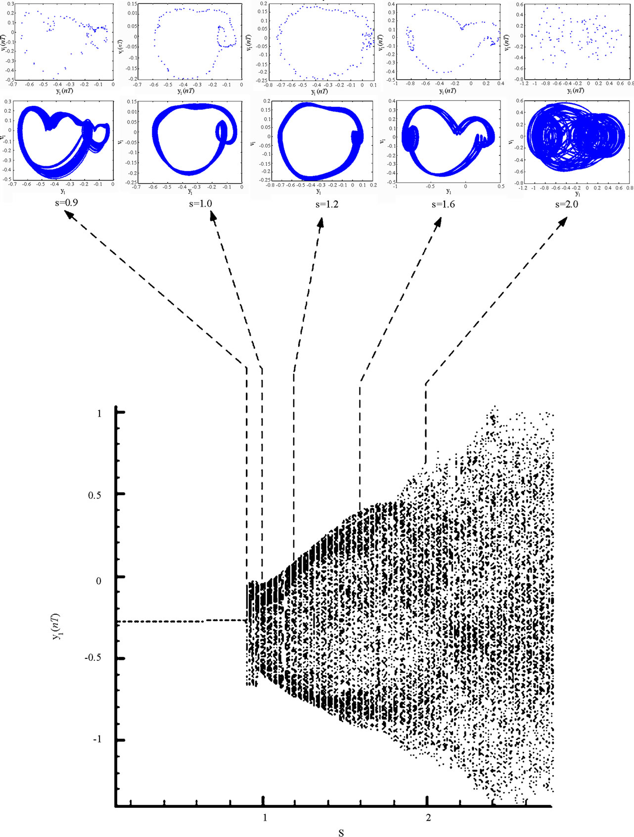
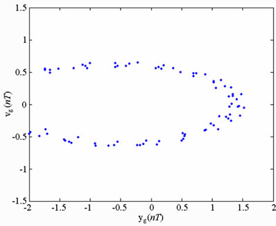
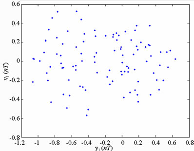
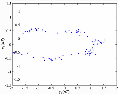
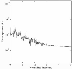
In practical bearing systems, the rotational speed ratio s is commonly used as a control parameter. Accordingly, the dynamic behavior of the current gear-bearing system was examined using the dimensionless rotational speed ratio s as a bifurcation control parameter. Figure 3 presents the bifurcation diagrams for the gear-bearing system displacement against the dimensionless rotational speed ratio, s and some dynamic trajectories and Poincaré maps (e.g. s = 0.9, 1.0, 1.2, 1.6 and 2.0) are exemplified to describe corresponding dynamic responses. The bifurcation diagrams show that the geometric center of gear and bearing perform synchronous 1T-periodic motion at low values of the rotational speed ratio, i.e. s < 0.9 and then the chaotic motion can be found as the dimensionless rotational speed ratio is increased over s = 0.9 for bearing center. Nevertheless, gear center performs quasi-periodic motion at s = 0.9. We may also make sure of the chaotic dynamic responses occurring for bearing center at i = 0.9 from observing the dynamic orbit (disordered trajectory) and Poincaré maps (irregularly-distributed points). At higher values of the dimensionless rotational speed ratio, i.e. s > 0.9, the dynamics of the centers of bearing 1 and bearing 2 behave as chaos, but gear center and pinion center are found to be quasi-periodic before the dimensionless rotational speed ratio s > 1.8. Then dynamic behavior of gear center and pinion center become chaotic while s ≥ 1.8. Therefore, we can find that the dynamic behaviors of geometric centers of bearing 1 (or bearing 2) and gear (or pinion) are not synchronous at higher rotational speed ratios, but persist periodic and synchronous at low rotational speed. Above results also prove that we will not be able to distinguish dynamic behaviors to be chaotic or quasi-periodic motions only by dynamic orbits or bifurcation diagrams, but also use other schemes such as Poincaré maps, Lyapunov exponent or fractal dimension to specify our dynamic responses. Thus we introduce Figure 4-7, i.e. phase diagram, power spectrum, Poincaré Map, Lyapunov exponent and fractal dimension for  and
and  with s = 1.8 and s = 2.0, and we can find the simulation results are corresponding with one another. Phase diagrams show disordered dynamic behaviors; power spectra reveal numerous excitation frequencies; the return points in the Poincaré maps form geometrically fractal structures; the maximum Lyapunov exponent is positive; the fractal dimensions are found to be 1.57 for
  at s = 1.8, 1.38 for
  at s = 1.8, 1.82 for
  at s = 2.0 and 1.46 for
  at s = 2.0.
Figure 8 present the bifurcation diagrams for the dimensionless displacement in the vertical direction of the gear-bearing system using the dimensionless unbalance coefficient β as a bifurcation parameter. It can be observed that the gear system exhibits chaotic motion at low values of the dimensionless unbalance coefficient, i.e. . However, as β is increased from 0.11, nonperiodic motion is replaced by the sub-synchronous nTperiodic motion. To test for the existence of a chaotic behavior at the values of the dimensionless unbalance coefficient, Figures 9-12 illustrate the phase diagrams, power spectra, Poincaré maps and Lyapunov exponents for the bearing center and gear center in the vertical direction of the gear-bearing system at β = 0.06 and 0.08, respectively. In every case, the phase diagrams are highly disordered and the power spectra reveal numerous excitation frequencies. Furthermore, it can be seen that the return points in the Poincaré maps form geometrically fractal structures and the maximum Lyapunov exponent is positive in each case. In other words, the results presented in these figures all indicate that the gear center exhibits a chaotic behavior at the values of the dimensionless unbalance coefficient (β = 0.06 and 0.08). We may conclude and prove that greater unbalance parameters would be able to suppress non-periodic motions to be nT-periodic motions and even escape the undesired motions.
5. Conclusion
This study has presented a numerical analysis of the nonlinear dynamic response of a gear-bearing system subject to nonlinear suspension effects, turbulent flow effect, long journal bearing, nonlinear oil-film force and nonlinear gear mesh force. The dynamics of the system
 (a)
(a) (b)
(b)
Figure 3. Bifurcation diagrams of gear-bearing system using dimensionless rotational speed ratio, s, as bifurcation parameter.
 (a)
(a) (b)
(b)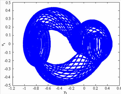 (c)
(c)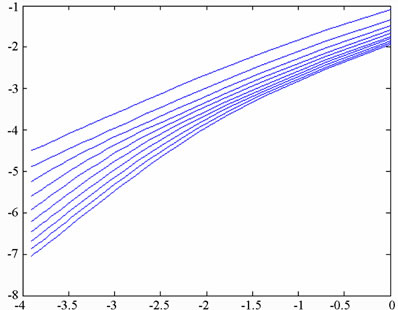 (d)
(d)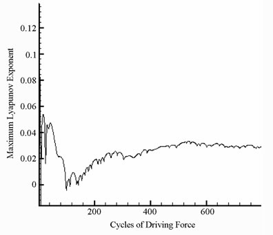 (e)
(e)
Figure 4. Simulation results obtained for gear-bearing system with s = 1.8(y1).
 (a)
(a) (b)
(b)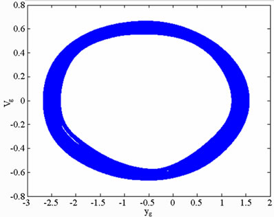 (c)
(c)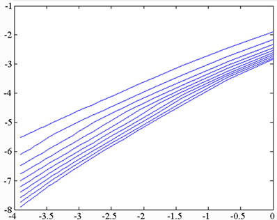 (d)
(d) (e)
(e)
Figure 5. Simulation results obtained for gear-bearing system with s = 1.8(y1).
 (a)
(a)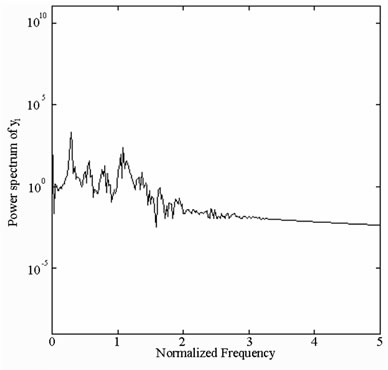 (b)
(b) (c)
(c)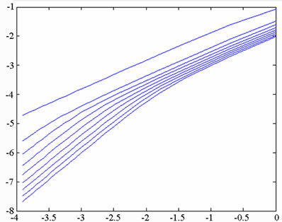 (d)
(d)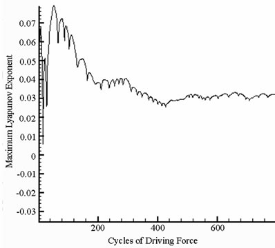 (e)
(e)
Figure 6. Simulation results obtained for gear-bearing system with s = 2.0(y1).
 (a)
(a) (b)
(b)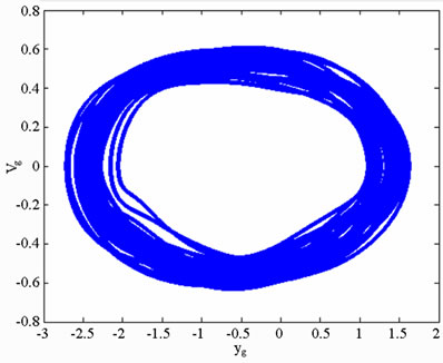 (c)
(c)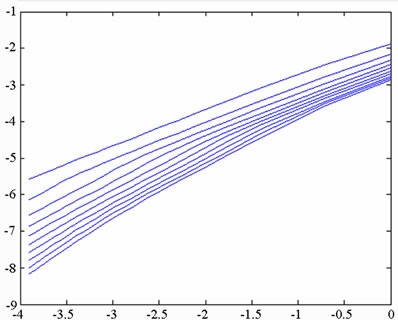 (d)
(d) (e)
(e)
Figure 7. Simulation results obtained for gear-bearing system with s = 2.0(y1).
 (a)
(a)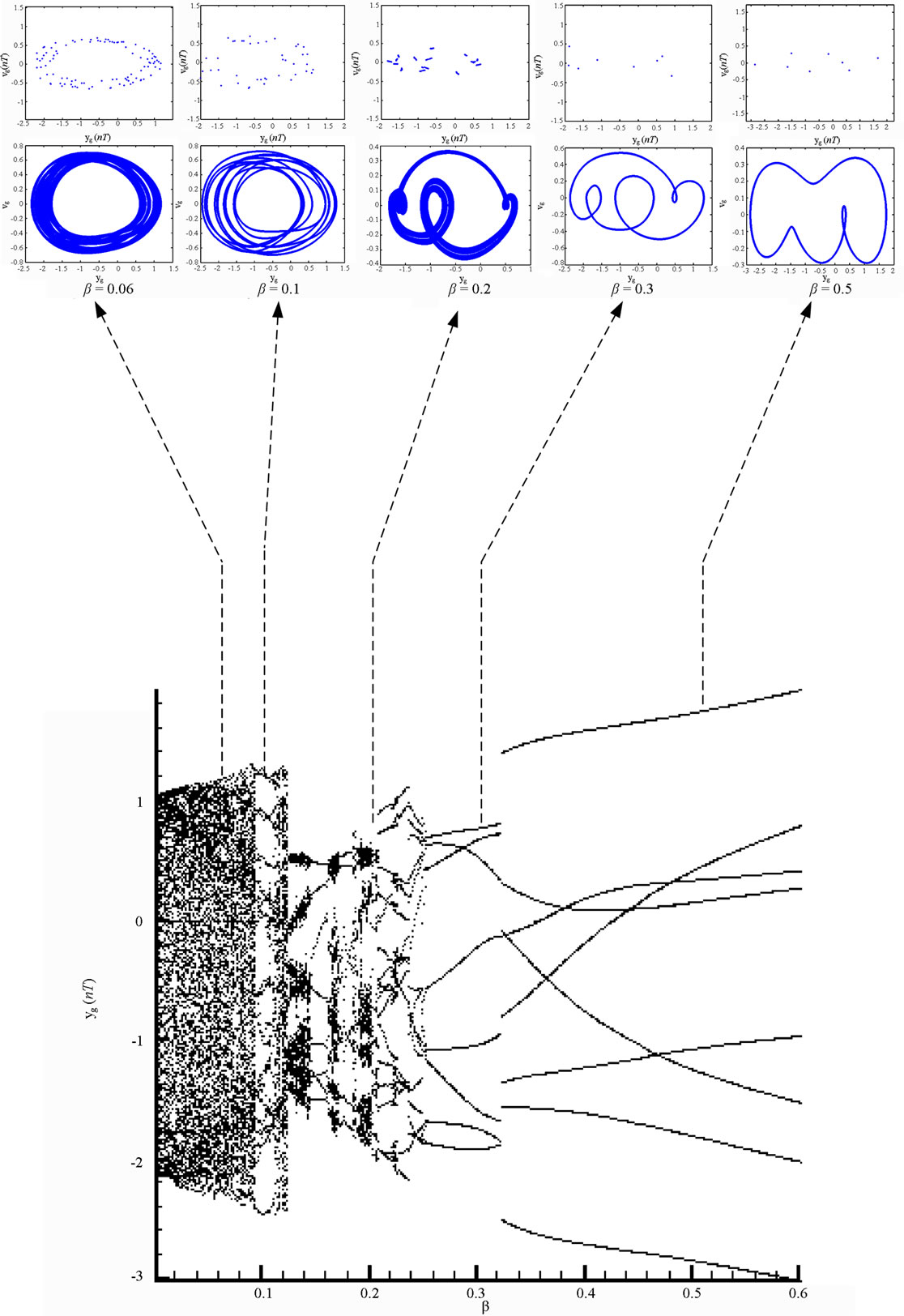 (b)
(b)
Figure 8. Bifurcation diagrams of gear-bearing system using dimensionless unbalance parameter, β, as bifurcation parameter.
 (a)
(a) (b)
(b) (c)
(c) (d)
(d)
Figure 9. Simulation results obtained for gear-bearing system with β = 0.06(y1).
 (a)
(a)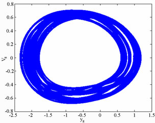 (b)
(b)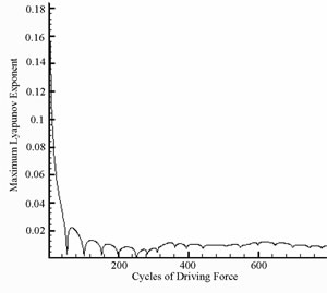 (c)
(c)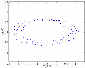 (d)
(d)
Figure 10. Simulation results obtained for gear-bearing system with β = 0.06(y1).
have been analyzed by reference to its dynamic trajectories, power spectra, Poincaré maps, bifurcation diagrams, maximum Lyapunov exponents and fractal dimensions. The analysis has investigated the dynamic response of the gear-bearing system as a function of both the dimensionless unbalance coefficient and the dimensionless rotational speed ratio. Overall, the results presented in this study provide a detailed understanding of the nonlinear
 (a)
(a)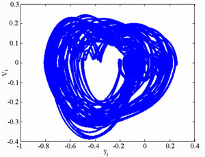 (b)
(b) (c)
(c)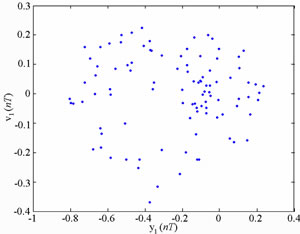 (d)
(d)
Figure 11. Simulation results obtained for gear-bearing system with β = 0.08(y1).
 (a)
(a)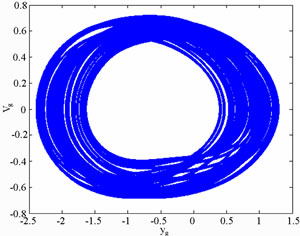 (b)
(b) (c)
(c)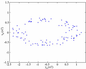 (d)
(d)
Figure 12. Simulation results obtained for gear-bearing system with β = 0.08(y1).
dynamic response of a gear-bearing system under typical unbalance approximations and rotational speed conditions. Specifically, the results enable suitable values of the unbalance coefficient and rotational speed ratio to be specified such that chaotic behavior can be avoided, thus reducing the amplitude of the vibration within the system and extending the system life even for turbulent flow approximation.
6. Acknowledgements
We would also like to thank the National Science Council of the Republic of China for supporting this project under contract No. NSC101-2221-E-214-014.
REFERENCES
- L. Vedmar and A. Anersson, “A Method to Determine Dynamic Loads on Spur Gear Teeth and on Bearings,” Journal of Sound and Vibration, Vol. 267, No. 5, 2003, pp. 1065-1084. doi:10.1016/S0022-460X(03)00358-4
- A. Kahraman and R. Singh, “Nonlinear Dynamics of a Spur Gear Pair,” Journal of Sound and Vibration, Vol. 142, No. 1, 1990, pp. 49-75. doi:10.1016/0022-460X(90)90582-K
- H. H. Lin, R. L. Huston and J. J. Coy, “On Dynamic Loads in Parallel Shaft Transmission: Part 1—Modeling and Analysis,” Transactions of American Society of Mechanical Engineers, Journal of Mechanics Transformation Automation in Design, Vol. 110, No. 2, 1988, pp. 221-225.
- K. Y. Yoon and S. S. Rao, “Dynamic Load Analysis of Spur Gears Using a New Tooth Profile,” Transactions of American Society of Mechanical Engineers, Journal of Mechanics Transformation Automation in Design, Vol. 118, No. 1, 1996, pp. 1-6. doi:10.1115/1.2826851
- K. Ichimaru and F. Hirano, “Dynamic Behavior of HeavyLoaded Spur Gears,” Transactions of American Society of Mechanical Engineers, Journal of Engineering for Industry, Vol. 96, No. 2, 1974, pp. 373-381. doi:10.1115/1.3438339
- M. Amabili and A. Fregolent, “A Method to Identify Model Parameters and Gear Errors by Vibrations of a Spur Gear Pair,” Journal of Sound and Vibration, Vol. 214, No. 2, 1998, pp. 339-357. doi:10.1006/jsvi.1998.1587
- H. N. Ozguven and D. R. Houser, “Mathematical Models Used in Gear Dynamics,” Journal of Sound Vibration, Vol. 121, No. 3, 1988, pp. 383-411. doi:10.1016/S0022-460X(88)80365-1
- H. N. Ozguven and D. R. Houser, “Dynamic Analysis of High Speed Gears by Using Loaded Static Transmission Error,” Journal of Sound Vibration, Vol. 125, No. 1, 1988, pp. 71-83. doi:10.1016/0022-460X(88)90416-6
- Y. Cai and T. Hayashi, “The Linear Approximated Equation of Vibration of a Pair of Spur Gears,” Transactions of American Society of Mechanical Engineers, Journal of Mechanics Transformation Automation in Design, Vol. 116, No. 2, 1994, pp. 558-564. doi:10.1115/1.2919414
- K. Umezawa and S. T. Ishikawa, “Simulation on Rotational Vibration of Spur Gears,” Bulletin of the Japan Society of Mechanical Engineers, Vol. 27, 1984, pp. 102- 109.
- P. D. Mcfadden and M. M. Toozhy, “Application of Synchronous Averaging to Vibration Monitoring of Rolling Element Bearings,” Mechanical Systems and Signal Processing, Vol. 14, No. 6, 2000, pp. 891-906. doi:10.1006/mssp.2000.1290
- F. L. Litvin, Q. Lian and A. L. Kapelevich, “Asymmetric Modified Spur Gear Drives: Reduction of Noise, Localization of Contact, Simulation of Meshing and Stress Analysis,” Computer Methods in Applied Mechanics and Engineering, Vol. 188, No. 1-3, 2000, pp. 363-390. doi:10.1016/S0045-7825(99)00161-9
- Y. H. Guan, M. F. Li, T. C. Lim and W. S. Shepard, “Comparative Analysis of Actuator Concepts for Active Gear Pair Vibration Control,” Journal of Sound Vibration, Vol. 269, No. 1-2, 2004, pp. 273-294. doi:10.1016/S0022-460X(03)00072-5
- D. Giagopulos, C. Salpistis and S. Natsiavas, “Effect of Non-Linearities in the Identification and Fault Detection of Gear-Pair Systems,” International Journal of Nonlinear Mechanics, Vol. 41, No. 2, 2006, pp. 213-230. doi:10.1016/j.ijnonlinmec.2005.07.004
- S. Theodossiades and S. Natsiavas, “On Geared Rotordynamic Systems with Oil Journal Bearings,” Journal of Sound and Vibration, Vol. 243, No. 4, 2001, pp. 721-745. doi:10.1006/jsvi.2000.3430
- S. Theodossiades and S. Natsiavas, “Periodic and Chaotic Dynamics of Motor-Driven Gear-Pair Systems with Backlash,” Chaos, Solitons & Fractals, Vol. 12, No. 13, 2001, pp. 2427-2440. doi:10.1016/S0960-0779(00)00210-1
- V. N. Constantinescu, “Analysis of Bearings Operating in Turbulent Regime,” Journal of Basic Engineering, Vol. 84, No. 1, 1962, pp. 139-151. doi:10.1115/1.3657235
- H. G. Elrod and C. W. Ng, “A Theory for Turbulent Films and Its Application to Bearings,” Journal of Lubrication Technology, Vol. 86, 1967, pp. 346-362.
- G. G. Hirs, “A Bulk-Flow Theory for Turbulence in Lubricants Films,” Journal of Lubrication Technology, Vol. 95, No. 2, 1973, pp. 137-146. doi:10.1115/1.3451752
- H. Hashimoto, S. Wada and K. Nojima, “Performance Characteristics of Worn Journal Bearings in Both Laminar and Turbulent Regimes, Part I: Steady State Characteristics,” ASLE Transactions, Vol. 29, No. 4, 1986, pp. 565-571. doi:10.1080/05698198608981721
- H. Hashimoto, S. Wada and K. Nojima, “Performance Characteristics of Worn Journal Bearings in Both Laminar and Turbulent Regimes, Part II: Dynamic Characteristics,” ASLE Transactions, Vol. 29, No. 4, 1986, pp. 572- 577. doi:10.1080/05698198608981722
- G. Capone, M. Russo and R. Russo, “Dynamic Characteristics and Stability of a Journal Bearing in a NonLaminar Lubrication Regime,” Tribology International, Vol. 20, No. 5, 1987, pp. 255-260. doi:10.1016/0301-679X(87)90025-9
- A. Kumar and S. S. Mishra, “Stability of a Rigid Rotor in Turbulent Hydrodynamic Worn Journal Bearings,” Wear, Vol. 193, No. 1, 1996, pp. 25-30. doi:10.1016/0043-1648(95)06654-3
- M. Lahmar, A. Haddad and D. Nicolas, “An Optimized Short Bearing Theory for Nonlinear Dynamic Analysis of Turbulent Journal Bearings,” European Journal of Mechanics A/Solids, Vol. 19, No. 1, 2000, pp. 151-177. doi:10.1016/S0997-7538(00)00139-X
- C. W. Chang-Jian and C. K. Chen, “Bifurcation and Chaos of a Flexible Rotor Supported by Turbulent Journal Bearings with Non-linear Suspension,” Transactions of IMechE Part J: Journal of Engineering Tribology, Vol. 220, No. 6, 2006, pp. 549-561. doi:10.1243/13506501JET167
- P. Grassberger and I. Proccacia, “Characterization of Strange Attractors,” Physical Review Letter, Vol. 50, No. 5, 1983, pp. 346-349. doi:10.1103/PhysRevLett.50.346
- C. L. Chen and H. T. Yau, “Chaos in the Imbalance Response of a Flexible Rotor Supported by Oil Film Bearings with Non-Linear Suspension,” Nonlinear Dynamics, Vol. 16, No. 1, 1998, pp. 71-90. doi:10.1023/A:1008239206153