World Journal of Mechanics
Vol.2 No.1(2012), Article ID:17681,9 pages DOI:10.4236/wjm.2012.21003
The Mesoscopic Constitutive Equations for Polymeric Fluids and Some Examples of Viscometric Flows*
Department of Mathematics, Altai State Technical University, Barnaul, Russia
Email: pyshnograi@mail.ru
Received November 6, 2011; revised December 5, 2011; accepted December 17, 2011
Keywords: Rheology; Linear Polymer Melts and Solutions; Constitutive Equation; Mesoscopic Approach
ABSTRACT
Constitutive equations for melts and concentrated solutions of linear polymers are derived as consequences of dynamics of a separate macromolecule. The model is investigated for viscometric flows. It was shown that the model gives a good description of non-linear effects of simple shear polymer flows: viscosity anomalies, first and second normal stresses, non-steady shear stresses.
1. Introduction
Describing viscoelastic behavior of the polymer system, one should distinguish the case of highly concentrated (c > 10%) solutions and melts of long polymers—strongly entangled systems ( ), where
  is the length (in any units) of a macromolecule and
  is the length of a part of macromolecule between the adjacent entanglements [1-3], and the case of melts of shorter polymers and half-dilute polymer solutions (c ~ 1% - 10%)— weakly entangled systems (
 ) [4]. The convenient characteristic of a system of entangled linear macromolecules (solutions and melts of polymers) appears to be
 , which, for strongly entangled systems, is inversely proportional to number of entanglements for one macromolecule—
 . Here
  is the polymer density. The quantity
  can be easily with estimated the value
  of real component of dynamic modulus
  on the typical plateau, according to the formula for weakly and strongly entangled systems, correspondingly
 .
.
In this paper we consider the case of weakly entangled systems and formulate a rheological equation of state (RES) that establishes a relationship between the stress tensor, kinetic characteristics, and internal dynamic parameters. At present, a large number of such equations of various complexity is known for polymeric liquids, but, despite various approaches both phenomenological [5-7] and microstructural [1,2,8-11] ones, the problem how to include specific features of a polymer system into the form of constitutive equations has no complete solution. This is due to both complexity of these systems, which are formed by tangled macromolecules, and mathematical difficulties [11]. The information about the microstructure and micro dynamics of the material ought to be incorporated into the present theory of linear and nonlinear relaxation phenomena in polymer systems. An advantage of the micro structural approach is a possibility of studying the relationship between the micro characteristics of a polymer system (concentration and molecular weight of the polymer) and macroscopically observed quantities (viscosity, shear and normal stresses, etc.). In this connection using microstructural concepts it’s feasible to formulate a sequence of RES that takes into account new molecular effects in each stage. At [4,9,12] obtained and studied a simple rheological model which can be chosen as an initial approximation in formulating such a sequence of RES. In this work, RES [4] is extended to the case of allowance for the additional corrections caused by intrinsic viscosity and the delayed interaction of a macromolecule with its environment. Realization of this approach involves consequent solution of two problems: formulation of the equations of dynamics for a macromolecule and transition from the formulated equations to RES. The resulting equations can be recommended as the first approximation in constructing a sequence of RES. Comparison of the approach with others, Graessley [1,3] and Doi-Edwards [8] approaches, one can find in [9,12].
2. Dynamics of a Macromolecule in Flow
The mesoscopic approach to the description of the dynamics of polymer systems is based on the equations of the macromolecule dynamics which cannot be formulated without additional assumptions, namely:
1) A monomolecular approximation of the system. It means that, instead of the entire set of interacting macromolecules in the volume we consider are non-interacting separate macromolecule, moving in the effective medium formed by the solvent and the other macromolecules.
2) The coarse-grained approximation of a macromolecule. It means that, irrespective of the chemical nature of the polymer, the slow motions of the chosen macromolecule can be described as motions of N centers of friction (beads) connected by elastic entropy forces (springs) in a chain. These assumptions lead to the following equations of the macromolecules dynamics [9] in normal modes:
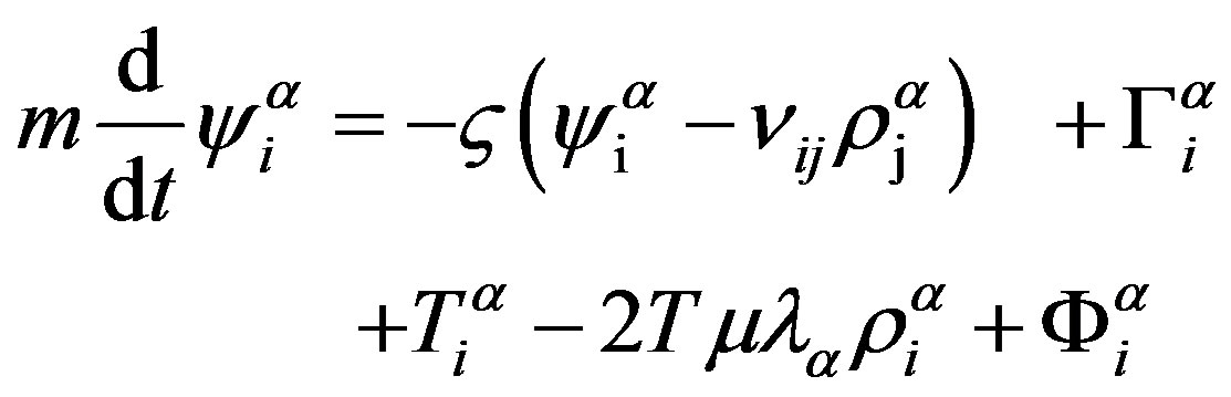 , (1)
, (1)
where  and
and 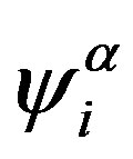 are the i-th components of the normal coordinates and velocity,
  is the mass of a bead. Here
 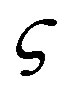 is the friction coefficient of a bead in a monomer fluid,
  is the velocity-gradient tensor, which is conveniently expressed below as the sum of symmetric
  and anti-symmetric
  parts, and the bracketed expression is the difference between the particle velocity at a given point of space and the velocity of undisturbed flow at this point. The force
  describes the interaction of the polymer chain with the environment via the solvent, while the force
  is an intrinsic resistance force,
  is a random force, and
  is the coefficient of elasticity.
Expression (1) is the basis for the description of the dynamics for different polymer systems [12]. The definition of the extra forces  and
and  allows one to specify the polymer system. Different models of these forces correspond to different physical cases. For dilute polymer solutions, in which polymer macromolecules can be considered non-interacting, the extra forces are considered to be equal to zero [9]. In concentrated polymer systems, the macromolecules cannot be considered as not interacting. So, one has to take into account the reaction of the environment and the strengthening of the friction coefficient. The first factor is due to the delayed character of interaction of the macromolecule with its environment, and the second is due to the fact that the chosen bead undergoes resistance not only from the monomer solvent, but also from other macromolecules. Furthermore, one should take into account that, in the flow with nonzero velocity gradients, a macromolecular coil changes its form, and the medium, formed by the coils becomes anisotropic. This mobility anisotropy of beads is called induced and is determined by the shape and orientation of macromolecular coils [4,9,12]. According to all these factors the equation for the force of hydrodynamic entrainment follows:
 (2)
(2)
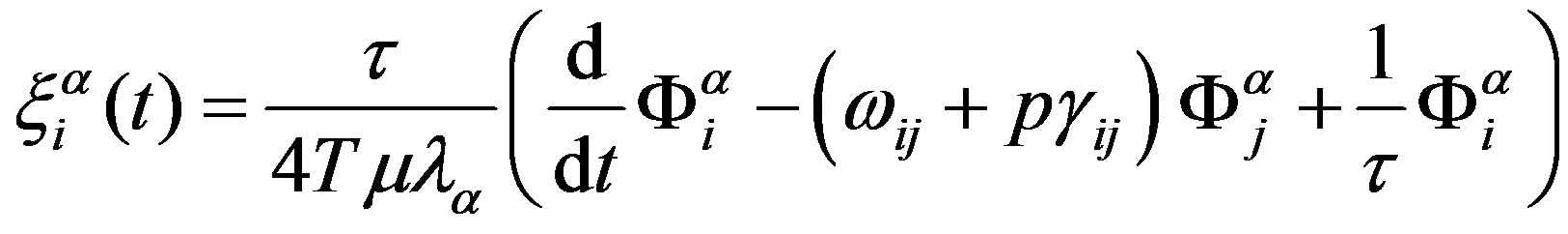
Here  is the relaxation time of the environment,
  is the dimensionless tensor friction coefficient of a bead,
  is the strengthening measure of the friction coefficient
 , and
, and  is a parameter. The bracketed expression on the left side of (2) is a substantial derivative of the vector quantity
  [9]. The presence of this derivative allows one to meet the principle of material objectivity in Equation (2) [6,9]. Numerical parameter
  entering into the definition of the substantial derivative can take different values. For
  = 0, the substantial derivative becomes the Jaumann derivative which has a simpler form while for
  = 1 and –1, it becomes the upper and lower convective derivatives, respectively. The specific value of
  corresponding to one of the above-mentioned derivatives in (2) is determined below.
If macromolecules form a tangled system besides the force of hydrodynamic entrainment, one should take into account the intrinsic viscous force , the meaning of which is elucidated by Pokrovskii et al. [12]. The specific requirement imposed on the force
  is that this force is vanishing when a macromolecular coil is rotating as a unit. All this allows one to write the equation for this force in similar to (2) manner in the form
 , (3)
, (3)
where:  is the dimensionless tensor friction coefficient and
  is the strengthening measure of the friction coefficient
  for the intrinsic viscous force
 . Intrinsic viscous force
  (since
 ) has relaxation character and depends on the anisotropic properties of the environment.
We assume that the anisotropy of mobility in considered polymer system is characterized by the second-order symmetric tensor . Then, for coefficients
  and
and  we write [9]
 (4)
(4)
Thus, (1-4) is the system of equations of dynamics of a macromolecule. The random force  entering into (1) is the Gaussian random process with a zero average. Its correlation tensor satisfies the corresponding fluctuation-dissipation relation [9,10].
3. Stress Tensor and Rheological Equation of State
Equations (1)-(4) give a microscopic picture of a polymer system flow based on discrete variables. Transition to the continuous case, i.e., to the description of polymer-system flows in terms of continuum mechanics, requires introduction of macroscopic variables—density  and momentum density
 . These variables are introduced in the standard manner [9,11]:
 (5)
(5)
Here  and
and  are vectors of position and velocity of the bead with number
 ,
,  is the co-ordinate vector of the chosen point in space, and
  is time. Sum is taken over all beads in a unit volume, and averaging is performed over the ensemble of all possible realizations of the random force
 .
.
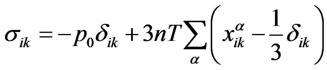
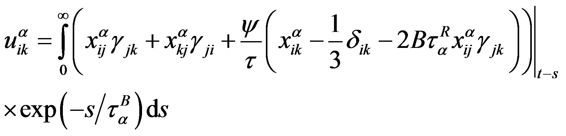
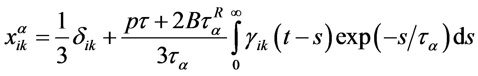
Differentiating (5) due to time yields an equation of mass conservation, and transformation to generalized coordinates using (1) yields an equation for momentum density. In the latter case, we have an expression for the stress tensor of a polymer system in terms of statistical characteristics of the system (1-4) solutions:
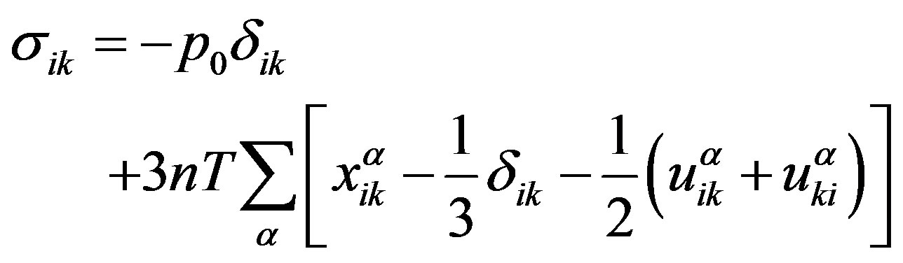 , (6)
, (6)
where  is pressure, n is the number of macromolecules in a volume unit, T is the temperature in energy unitsand
  and
and 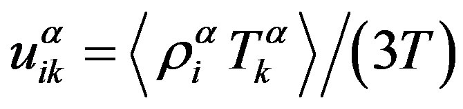
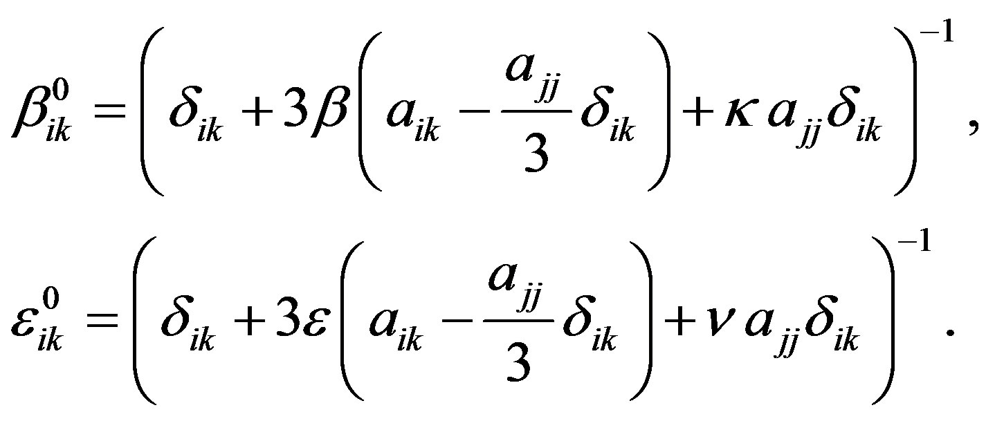
are internal thermodynamic parameters with equilibrium values
 ,
, (7)
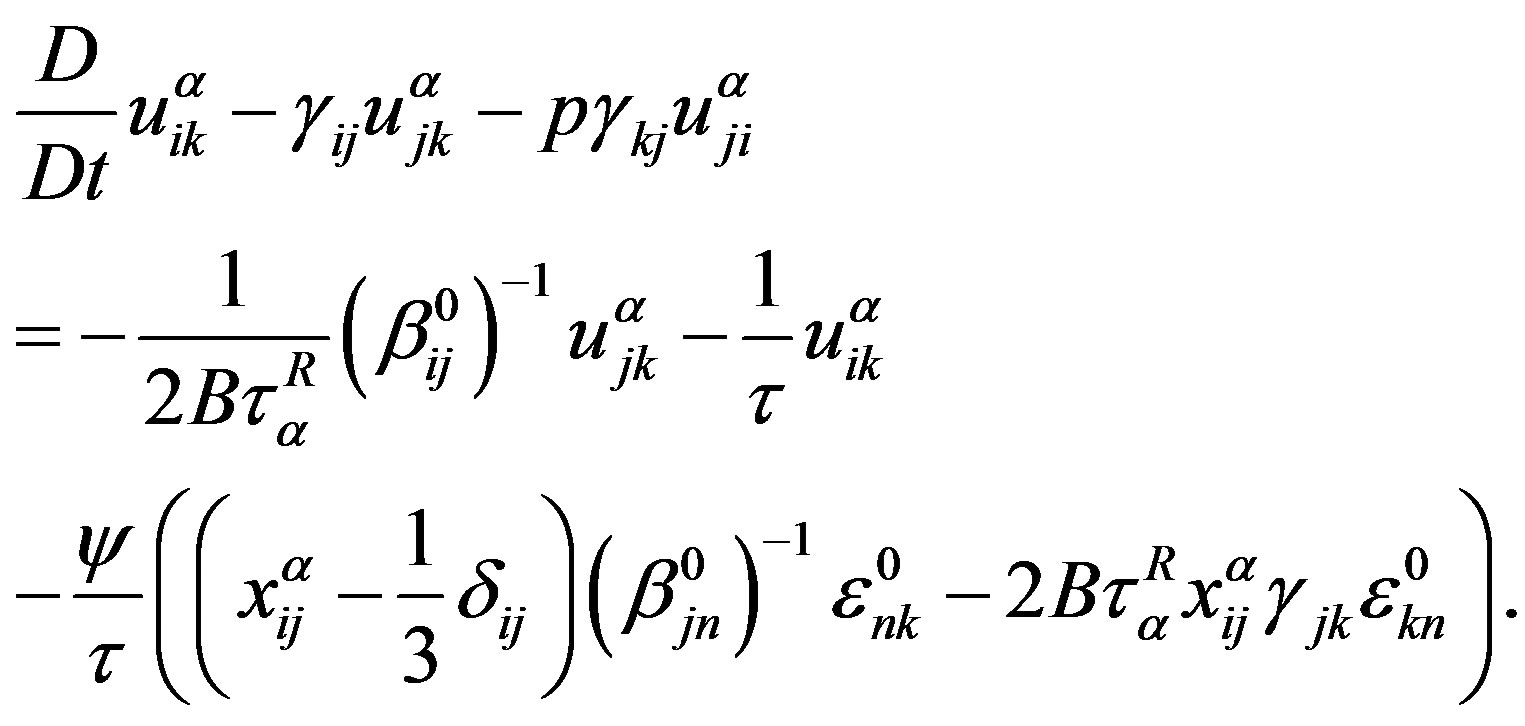
(7)
In the inertia-free case (m = 0), one can formulate (see Appendix) the relaxation equations for the dimensionless correlation moments  and
and  in the following form
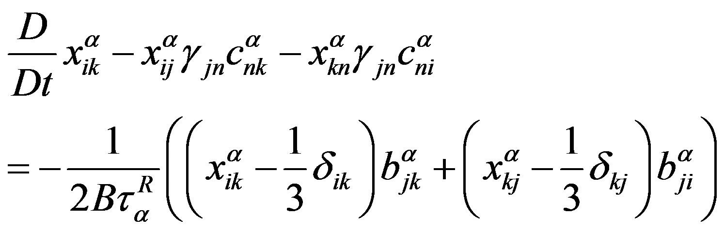 , (8)
, (8)
 , (9)
, (9)
where: 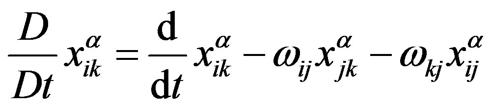 is the Jaumann derivative of the tensor quantity
  and
and  is the measure of intrinsic viscosity,
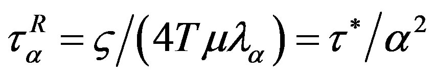
is a set of the Rouse relaxation times. In Equations (8)-(9) symbols  are used.
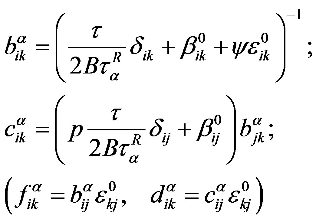 (10)
(10)
Thermodynamic variables  entering into (6) characterize the inertial properties of a macromolecular coil and, hence, can be used to determine anisotropy tensor
  in (4). Following [9], we write
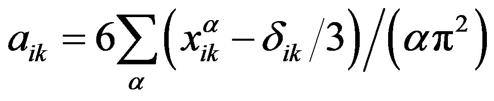 .
.
Therefore it becomes possible to establish the physical meaning of the microanisotropy parameters entering into (4). These parameters take into account dimensions  and shape
  of a macromolecular coil in the equations for macromolecule dynamics.
The Equations (6), (8), and (9) define a nonlinear, anisotropic, viscoelastic fluid. The behavior of system (6), (8), and (9) is determined by the six dimensionless parameters ( ,
,  ,
,  ,
,  ,
,  , and
, and ) and two dimensional parameters (
 and
and ). Parameter
  characterizing the ratio of the relaxation time of the environment
  to the maximum relaxation time
  was estimated in [9], where it was shown that
  for sufficiently long polymer chains. As to parameter
 , here two cases can be distinguished:
  [13,14-16] and
  [5], which are discussed below. As in [13], it is convenient to consider simpler forms of equations (8) and (9) by using the smallness of the parameters
  and
and . We consider in more detail the case
 , which corresponds to the dynamics of polymer solutions at a concentration about of 1%.
Considering only effects of the first order with respect to  and
and , we note that Equations (6) and (8) do not change, and Equation (9) takes the form
 (11)
(11)
In the zero-th approximation for  and
and , variable
  and Equations (6) and (8) take the form
 , (12)
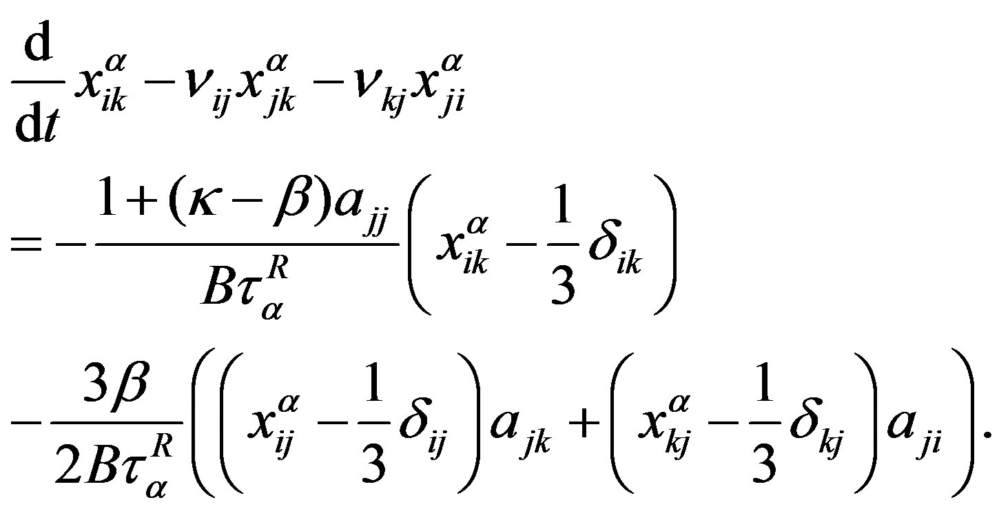
The parameters of this system are ,
,  , and
, and . Note that when
  = 1, system (12) is the system of equations for a dumbbell model
 , (13)
where  and
and  are the initial shear viscosity and the relaxation time, and
 . The system (13) under the assumption of isotropic relaxation (
 = 0), is followed by the well-known structural phenomenological Vinogradov-Pokrovskii model [13,14-17].
The model (13) is simple and gives high accuracy in describing steady nonlinear effects, though it is only the zero-order approximation model, which does not permit one to predict all features of polymer flow. In case, one needs more details, one can consider the contributions of parameters  and
and  which take into account the relaxation character of the environment and the intrinsic viscosity in the equations for macromolecule dynamics.
4. Linear Effects of the Rheological Model
To obtain an expression for the dynamic shear modulus that corresponds to system (6), (8), and (9), we find a solution to this system in a linear approximation with respect to the velocity gradients. In this case, anisotropy tensor  is equal to zero, and the terms
  can be omitted. Then (8) and (9) are written as
 ,
,

where ;
; 
The latter equations can be written as
 (14)
(14)
Solving the first equation of (14) by the method of successive approximations with first-order approximation due to the velocity gradients, we obtain
 .
.
Substitution of this expression into the second equation in (14) yields

In the simple oscillating shear flow  and the last two expressions together with (6) define the complex shear modulus
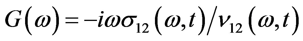
 (15)
(15)
Next, it is convenient to distinguish the real and imaginary parts in :
: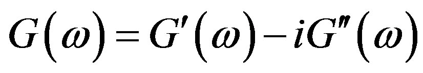 .
.
If the value of the modulus on the plateau is determined by (15), then
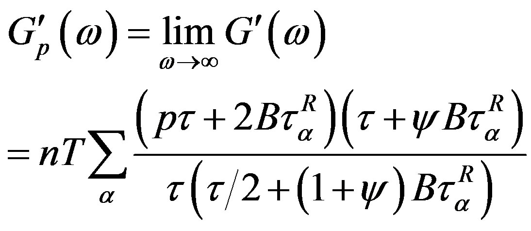 . (16)
This series converges only for p = 0. Thus, the Jaumann derivative in the equations of dynamics of a macromolecule (2) and (3) corresponds to cases a) and b). The definitions of the relaxation times ,
,  , and
, and  are given through parameters
  and
and , estimates of which are given in [4,9], where it was shown that, for sufficiently long chains, one can always assume
 . As to intrinsic viscosity parameter
 , here two alternative cases
  and
and  are distinguished.
The curves of  and
and  versus the dimensionless frequency
  calculated by (18) are given in Figures 1-4, from which one can see that the values of
  and
and  are mainly determined by parameter
 , and the impact of parameter
  (for
(for ) is insignificant. The existence of characteristic plateau is determined by relaxation time
 . In the case, when
  = 0, that corresponds to dilute solutions, irrespective of the type of convective derivative, a plateau on
  is absent. For
 , which corresponds to the dynamics of melts and strongly concentrated solutions [4], from (16) we have
 . The calculation results show that, for
 , the modulus on the plateau
 .
.
Therefore, the non-dependence of  on the molecular weight of a polymer means
 . Using the estimate for
  obtained in [11], from the last relation one can obtain
 .
.
The value of the initial shear viscosity , which can be expressed from (16) as

Figure 1. The contribution of parameter  to the dimensionless frequency dependence of real component of dynamic modulus
 .
.
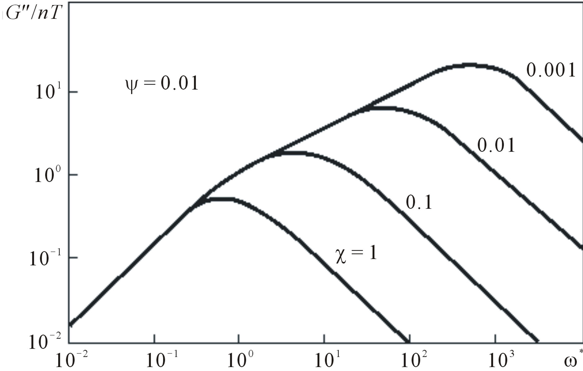
Figure 2. The contribution of parameter  to the dimensionless frequency dependence of imaginary component of dynamic modulus
 .
.
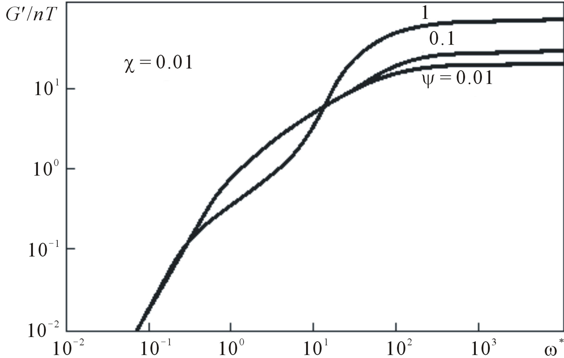
Figure 3. The contribution of parameter  (internal viscosity) to the dimensionless frequency dependence of real component of dynamic modulus
 .
.

Figure 4. The contribution of parameter  (internal viscosity) to the dimensionless frequency dependence of imaginary component of dynamic modulus
 .
.
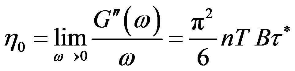 . (17)
To compare the calculation and experimental results, we turn to the data of Menezes and Graessley [16,17], where  and
and  were measured for solutions of polybutadiene with different molecular weights at the same concentration of c = 0.0676 g/cm. The above formulae allow us to find the following estimates of the parameters of the rheological model (6), (8), and (9) were obtained:
  = 0.077; 0.025; 0.011 and 0.005,
  = 0.21; 2.35; 16.27 and 147 sec, and
  = 840.4; 480.2; 321.5 and 206.7 Pa for molecular weights
  , respectively. In all cases,
  = 0.025. The comparison of the results is given in Figures 5 and 6, from which one can see satisfactory agreement between the theoretical and experimental curves of
  and
and  for
for  < 10 sec–1. The values of
  as a function of
  are given on Figure 7 showing good agreement with (17).
Figure 7 presents parameter  dependence molecular weight corresponding
 .
.
5. Non Linear Effects in the Simple Shear Flow
The system of constitutive Equations (6), (8), and (9) should be checked for correspondence to polymer fluid
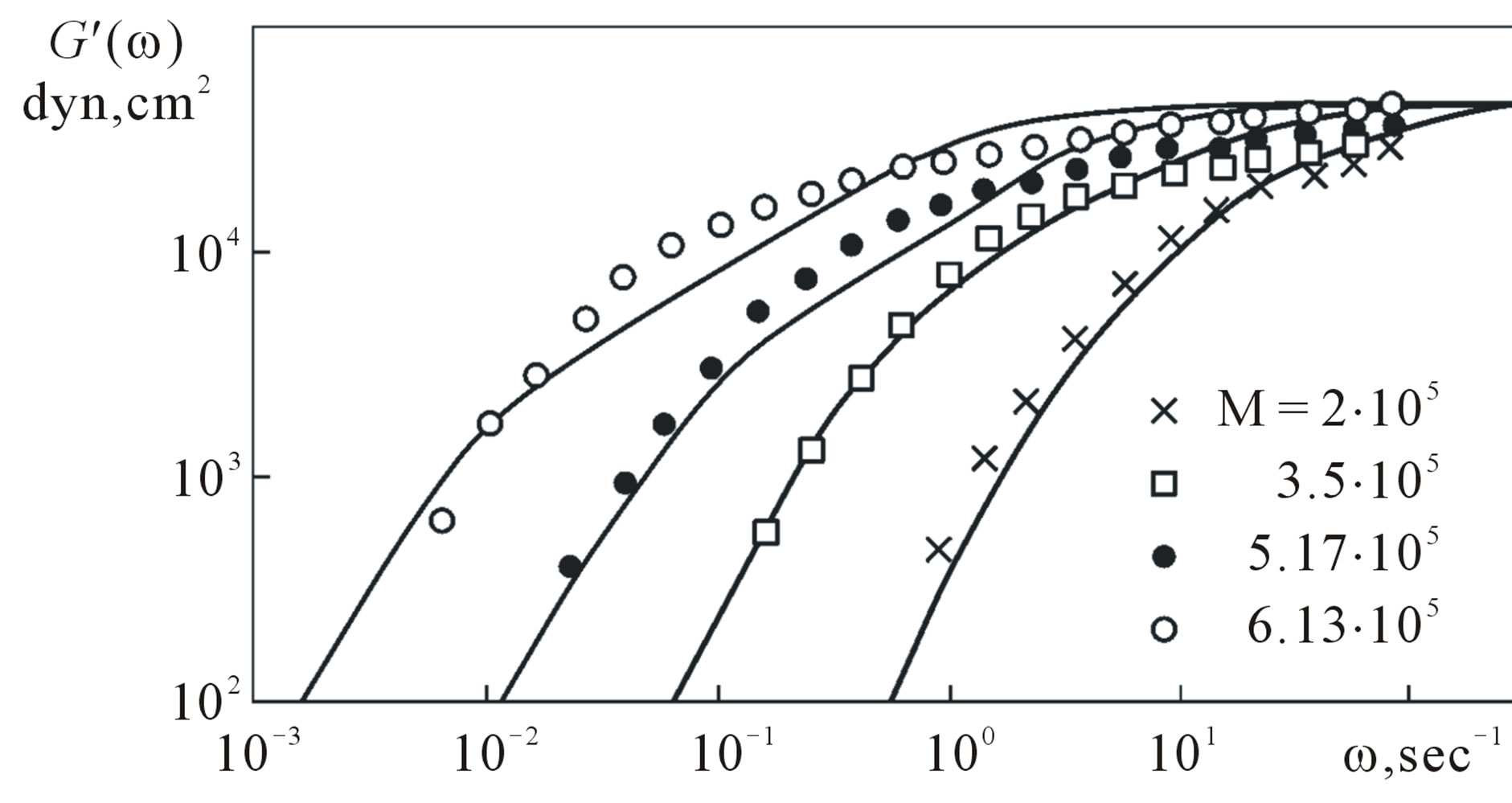
Figure 5. Real component of dynamic modulus  for polybutadiene solutions of various molecular weights (points) [16,17], compared with the predictions of Equation (15) (solid lines).
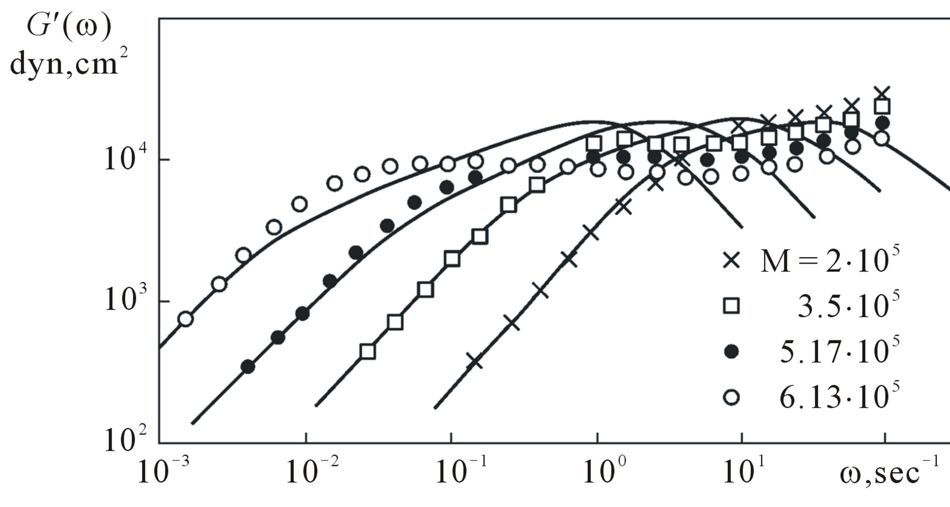
Figure 6. Imaginary component of dynamic modulus  for polybutadiene solutions of various molecular weights (points) [16,17], compared with the predictions of Equation (15) (solid lines).

Figure 7. Parameter dependence on molecular weight.
flows. Diverse flows leads to difficult mathematical problems and, naturally, the check of the RES should be start with the simplest cases. One type of flows that are often realized in viscometers of various design is simple shear. In this case, the velocity-gradient tensor contains only one nonzero component , which varies with time due to a well-known law. In steady flow, the gradient of velocity is constant, and rheological behavior of the polymer system is conveniently characterized by the following viscometric functions: shear viscosity
  and first
  and second
  normal stresses differences, which are given by
 (18)
(18)
The dependence  is often given in the form
 or
or . Here
  is the shear velocity and
  is the unit function of Heaviside. In the first case, system (6), (8), and (9) describes the establishment of stresses from the state of rest, and the corresponding viscometric functions (18) are denoted by
  and
and . In the second case, this system describes stress relaxation after shear deformation, and functions are denoted by
  and
and  and are generally functions of the velocity gradient and time. The following relations are apparently valid
 (19)
(19)
Solving (8) for case of a simple shear flow with shear velocity  with third-order accuracy with respect to
 , for viscometric functions we obtain

Thus, the parameters  and
and  are responsible for the nonlinear properties of system (12). For simple shear,
  appears even in the second order with respect to the velocity gradients, and
  appears only in the third.
At low shear velocities, the second difference of normal stresses  is given by the formula
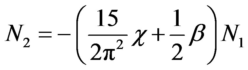 , (20)
obtained in [6]. Thus the model describes a non-zero second normal stress difference. The calculations show that, for , formula (20) remains valid for
  .
.
To compare RES (6), (8), and (9) with experiments, we use the data of Menezes and Graessley [16,17], who studied shear flows of polybutadiene solutions with various molecular weights. It is convenient to use their results, because their data on linear viscoelastictity have already been compared with (6), (8), and (9) in Section 4.
The results of the calculation for the viscometric functions (18) and the corresponding experimental values are given in Figures 8, 9 and 10. In the calculations, we used the following induced anisotropy parameters:  = 0.1,
  = 0.25,
  =0, and
  = 0.1. They were chosen from the condition of the best agreement between the theoretical curves and the experimental data. The value of
  was not measured in [16,17].
Let us consider nonlinear unsteady effects. The results of the calculation of the establishment of stresses for a
Figure 8. Experimental (solid lines) and theoretical (points) plots of the steady shear viscosity coefficient and the first difference of normal stresses vs. the shear velocity for various values of the molecular weight.
Figure 9. The comparison of experimental (solid lines) and theoretical (dashed lines) dependences of an establishment of stationary values of the shear viscosity coefficient and the first difference of normal stresses at various shear velocities.

Figure 10. The comparison of experimental (solid lines) and theoretical (dashed lines) dependences of relaxation of the shear viscosity coefficient and the first difference of normal stresses after shear deformation at various shear velocities.
specimen with  are given in Figure 9, which shows that Equations (2), (4), and (5) describes (the non-monotonic attainment of
  and
and  at high shear velocities. It is also found that
  and
and  at small t.
The data for  and
and  are given in Figure 10, which show that (18), (8) and (19) confirm the presence of two characteristic times for stress relaxation after intense shear deformation. The anisotropy parameter values are the same as in Figures 8 and 9.
6. Conclusion
Thus, the proposed microstructural approach to the description of the dynamics of polymer fluids does not contradict the available experimental data on the linear and non linear viscoelasticity of linear polymer solutions and melts. The obtained rheological equation of state is applicable for the description of steady and unsteady effects in both linear and nonlinear regions of strain rates and more complex flow regimes of linear polymer solutions and melts. The model can serve as a basis for the description of nonlinear effects in polymeric systems.
7. Acknowledgements
All authors thanks professor Vladimir Pokrovskii for the useful discussion.
REFERENCES
- W. W. Graessley, “The Constraint Release Concept in Polymer Rheology,” Advances in Polymer Science, Vol. 47, 1982, pp. 68-117.
- H. Watanabe, “Viscoelasticity and Dynamics of Entagled Polymers,” Progress in Polymer Science, Vol. 24, No. 9, 1999, pp. 1253-1403. doi:10.1016/S0079-6700(99)00029-5
- W. W. Graessley, “Polymeric Liquids & Networks: Dynamics and Rheology,” Garland Science, London, 2008.
- V. N. Pokrovskii, “The Mesoscopic Theory of Polymer Dynamics,” 2nd Edition, Springer, Berlin, 2010. doi:10.1007/978-90-481-2231-8
- J. D. Ferry, “Viscoelastic Properties of Polymars,” 3rd Edition, Wiley and Sons, London, 1980.
- A. Yu. Grosberg and A. R. Khokhlov, “Statistical Physics of Macromolecules,” Springer, Berlin, 1994.
- G. V. Pyshnograi, V. N. Pokrovskii, Yu. G. Yanovskii, Yu. N. Karnet and I. F. Obrazcov, “Equation of State for Nonlinear Viscoelastic (Polymer) Continua in Zero-Approximations by Molecular Theory Parameters and Secuentals for Shearing and Elongational Flows,” Doklady Russian Akademy Nauk, Vol. 335, No. 9, 1994, pp. 612- 615 (in Russian).
- M. Doi and S. F. Edwards, “The Theory of Polymer Dynamics,” Oxford University Press, Oxford, 1986.
- H. Ch. Ottinger, “Thermodynamically Admissible Reptation Models with Anisotropic Tube Cross Sections and Convective Constraint Release,” Journal of Non-Newtonian Fluid Mechanics, Vol. 89, No. 1-2, 2000, pp. 165- 185. doi:10.1016/S0377-0257(99)00025-7
- G. Astarita and G. Marucci, “Principles of Non-Newtonian Fluid Mechanics,” McGraw-Hill Inc., New York, 1974.
- A. I. Leonov, “A Brief Introduction to the Rheology of Polymeric Fluids,” Coxmoor Publishing Company, Oxford, 2008.
- A. Gusev, G. Afonin, I. Tretjakov and G. Pyshnogray, “The Mesoscopic Constitutive Equation for Polymeric Fluids and Some Examples of Flows,” In: N. P. Jennifer and M. L. Tyler, Eds., Viscoelasticity: Theories, Types and Models, Nova Publisher, New York, 2011, pp. 186-202.
- V. N. Pokrovskii, Yu. A. Altukhov and G. V. Pyshnograi, “On the Difference between Weakly and Strongly Entangled Linear Polymer,” Journal of Non-Newtonian Fluid Mechanics, Vol. 121, No. 2-3, 2004, pp. 73-86. doi:10.1016/j.jnnfm.2004.05.001
- Y. G. Yanovsky, V. N. Pokrovskii, Y. A. Altukhov and G. V. Pyshnograi, “Properties of Constitutive Equations for Undilute Linear Polymers Based on the Molecular Theory,” International Journal of Polymeric Materials, Vol. 36, No. 1-2, 1997, pp. 75-117.
- A. S. Gusev, G. V. Pyshnograi and V. N. Pokrovskii, “Constitutive Equations for Weakly Entangled Linear Polymers,” Journal of Non-Newtonian Fluid Mechanics, Vol. 163, No. 1-3, 2009, pp. 17-28.
- Yu. A. Altukhov, G. V. Pyshnograi and I. G. Pyshnograi, “Slipping Phenomenon in Polymeric Fluids Flow between Parallel Planes,” World Journal of Mechanics, 2011, Vol. 1, No. 6, pp. 294-298. doi:10.1016/S0377-0257(97)00116-X
- W. W. Graessley, “Polymeric Liquids & Networks: Dynamics and Rheology,” Garland Science, London, 2008.
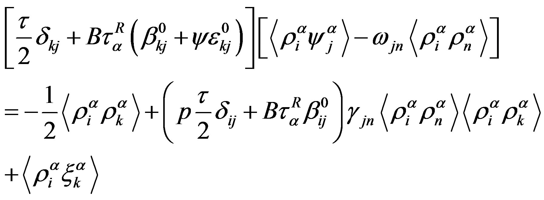
Appendix: Derivation of Relaxation Equations
We introduce relaxation equations for the dimensionless moments  and
and . In the inertia-free case (m = 0), Equations (1)-(4) can be written as
Here
 (A1)
(A1)
is a new random process which is  correlated [9],
  is a set of the Rouse relaxation times, and
  is the measure of intrinsic viscosity.
Using (8), we obtain a closed system of equations for the moments  and
and :
:
 , (A2)
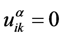
The moment  which is unknown in (A2), can be found from the fluctuation-dissipation theorem. Besides there is another method. The equilibrium values of the moments
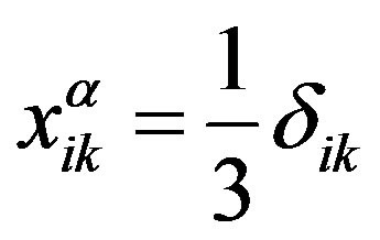
  and
and  were determined previously by Pokrovskii [6]:
 ,
,  (A3)
(A3)
These values should be obtained from (A2) at zero velocity gradients, and the moments  and
and  enter into (A2) in a linear manner. Hence, taking into account the desired moment
 , in (A2)
we should replace the moments  and
and 
that do not have the velocity-gradient tensor as a cofactor by  -
- and
and  -
- , respectively.
Going over to the dimensionless moments  in (9), we have
 , (A4)
where

is the Jaumann derivative of the tensor quantity .
.
Multiplying (A1) by  and averaging the resulting expression, we write the following equation for
 :
:
 . (A5)
We find the moment  entering into (A5) by multiplying (A1) by
  and performing averaging. Using (A3), we finally obtain
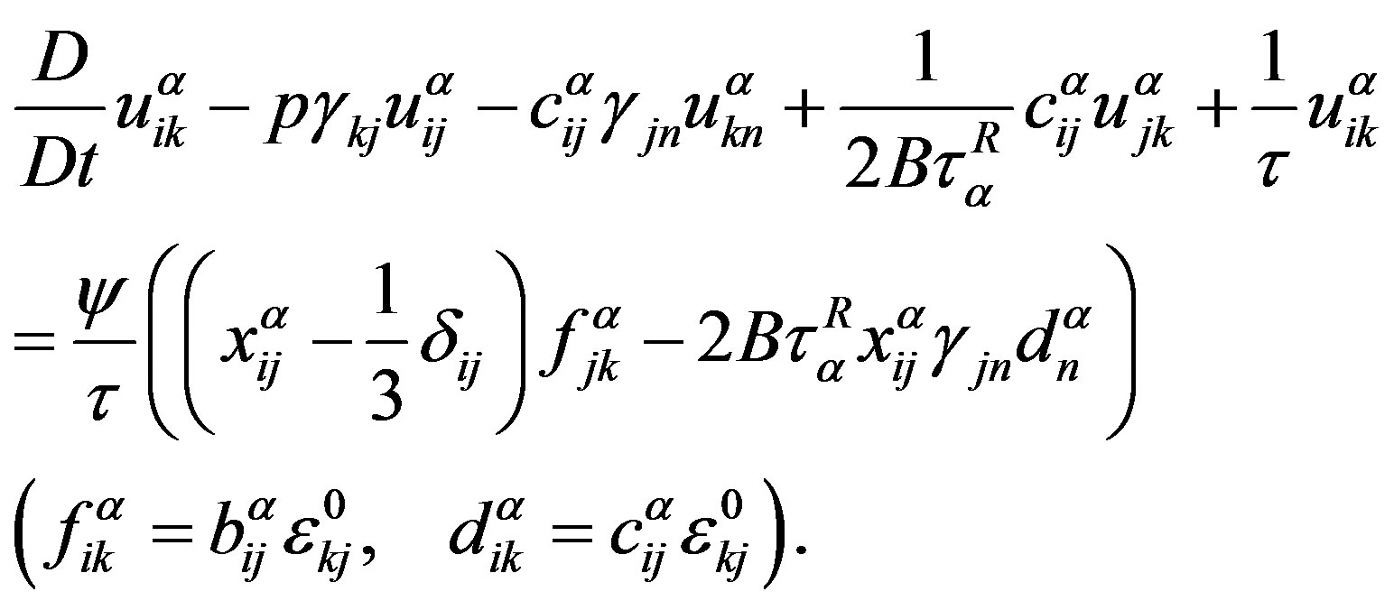 (A6)
(A6)
Since the expression for the stress tensor (6) is written in symmetric form, it is more convenient to use the variable 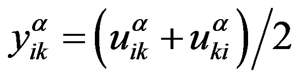 instead of
 . The equation for this variable can be obtained from (9) using the symmetry of tensors
 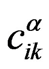 and
and  and assuming the permutability of tensors
  with
with ,
,  , and
, and . Assuming the existence functional relationship between
 ,
,  and
and  and also by virtue of the fact that
  and
and  are expressed in terms of
 , this assumption is not a significant constraint. Then, instead of (9), one obtains
 (A7)
(A7)
NOTES
*This work was supported by the Russian Foundation for Basic Research (Grant No. 09-01-00293).