World Journal of Mechanics
Vol. 1 No. 2 (2011) , Article ID: 4670 , 14 pages DOI:10.4236/wjm.2011.12005
An Efficient Numerical Method for Calculation of Elastic and Thermo-Elastic Fields in a Homogeneous Medium with Several Heterogeneous Inclusions
Mechanical Engineering Department, Instituto Tecnológico y de Estudios Superiores de Monterrey,
Campus Estado de México, Atizapan, Mexico
E-mail: kanaoun@itesm.mx
Received February 12, 2011; revised March 31, 2011; accepted April 8, 2011
Keywords: Elasticity, Heterogeneous Medium, Integral Equations, Gaussian Approximating Functions, Toeplitz Matrix, Fast Fourier Transform
ABSTRACT
The work is devoted to calculation of static elastic and thermo-elastic fields in a homogeneous medium with a finite number of isolated heterogeneous inclusions. Firstly, the problem is reduced to the solution of integral equations for strain and stress fields in the medium with inclusions. Then, Gaussian approximating functions are used for discretization of these equations. For such functions, the elements of the matrix of the discretized problem are calculated in explicit analytical forms. The method is mesh free, and only the coordinates of the approximating nodes are the geometrical information required in the method. If such nodes compose a regular grid, the matrix of the discretized problem obtains the Toeplitz properties. By the calculation of matrix-vector products with such matrices, the Fast Fourier Transform technique may be used. The latter accelerates essentially the process of the iterative solution of the disretized problem. The results of calculations of elastic fields in 3D-medium with an isolated spherical heterogeneous inclusion are compared with exact solutions. Examples of the calculation of elastic and thermo-elastic fields in the medium with several inclusions are presented.
1. Introduction
Calculation of elastic fields in homogeneous materials with isolated heterogeneous inclusions is an important problem of stress analysis of composites and materials with defects. Efficient numerical methods of the solution of this problem are based on the volume integral equations for the fields in heterogeneous media (see, e.g., [1-3]). By the use of these equations, the fields inside the inclusions become principal unknowns of the problem. If the fields inside the inclusions are known, the fields in the medium are reconstructed from the original integral equations. Thus, the problem should be solved only in the region occupied by the inclusions. This is the main advantage of the Integral Equation Method (IEM) over the Finite Element Method (FEM), where the fields in the medium as well as in the inclusions are equivalent unknowns, and the solution has to be found in the whole region. The IEM is preferable if inclusions being smaller than the characteristic sizes of the body are situated far from its boundary.
A conventional method of the solution of integral equations is based on the following procedure. The region of integration is divided into a finite number of sub-regions, where the unknown functions are approximated by some standard functions (e.g., polynomial splines, radial functions, wavelets, etc.). After application of the Method of Moments or the Collocation Method the problem is reduced to a finite system of linear algebraic equations with respect to the coefficients of the approximation (the discretized problem) (see, e.g., [3]). The elements of the matrix of this system are integrals over the sub-regions. For conventional approximating functions, a great portion of computer time is spent for numerical calculation of these integrals. The matrices of the discretized problems are usually non-sparse and have large dimensions (if high accuracy of the numerical solutions is required). Computational cost of the solution of linear algebraic systems with such matrices is rather high. In application to the 3D-integral equations of elasticity for a medium with inclusions, this traditional numerical scheme was carried out in [4,5].
In this work, an efficient numerical method for the solution of integral equations of elasticity and thermoelasticity for a 3D-homogeneous medium with a finite number of isolated inclusions is developed. For discretization of these equations, the Gaussian radial approximating functions are used. The theory of approximation by Gaussian and similar functions was developed in [6]. For such functions, the elements of the matrix of the discretized problems are calculated in explicit analytical forms. Thus, the time of the construction of this matrix is essentially reduced in comparison with the methods that incorporate conventional approximating functions and require numerical integration by the calculation of the matrix elements. For regular grids of approximating nodes, the matrix of the discretized problem has the Toeplitz structure, and the Fast Fourier Transform (FFT) technique may be used for the calculation of matrix-vector products in the process of iterative solution of the discretized problem. The initial “geometrical” information required in the method is only the coordinates of the approximating nodes but not detailed forms of the mesh cells. Thus, the method is mesh free in fact.
For the numerical solution of 2D-volume integral equations of elasticity, a similar method was developed in [7]. In the present work, the method is extended on the 3D-volume integral equations of elasticity and thermo elasticity.
The structure of this paper is as follows. In Section 2, the 3D-volume integral equations of elasticity for strain and stress fields in a homogeneous medium with a set of isolated heterogeneous inclusions are considered. In Section 3, Gaussian approximating functions are used for discretization of these equations. Comparisons of the numerical and exact solutions for a medium with a spherical inclusion which elastic properties vary along the radius are presented in Section 4. A medium with several isolated inclusions is also considered in this section. In Section 5, the problem of thermo-elasticity for the medium with inhomogeneities is considered. In the Conclusions, some details of the proposed method and the area of its application are discussed.
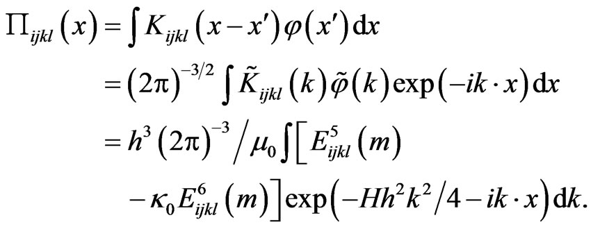
2. Integral Equations of Static Elasticity for a Homogeneous Medium with a Finite Number of Isolated Inclusions
Let an infinite homogeneous medium with the tensor of elastic constants  contain a finite number N of isolated inclusions that occupy regions
  (
( ). Elastic properties inside each region
  are defined by the tensors
 , where
 is a point of the 3D-space. The medium is subjected to an external strain
  (or stress
 ) field, and the objective is to calculate elastic strain and stress fields in the medium with the inclusions. This problem may be reduced to volume integral equations for the strain
  or stress
  tensors inside the inclusions. Let
 , and
, and  be the characteristic function of the region V occupied by the inclusions:
  if
if ,
,  if
if . The strain field
  in the medium with the inclusions satisfies the following integral equation (see, e.g., [1,8]):
 (1)
(1)
Here ,
,  when
when , and
, and  when
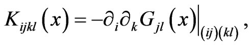
when . Summation with respect to repeating tensorial (low) indices is implied. The kernel
  of the integral operator in this equation is the second derivative of the Green function
  of the homogeneous host medium
 (2)
(2)
where  is the solution of the following equation:
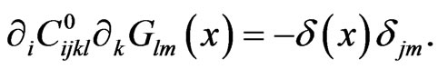 (3)
(3)
Here  is Kronecker’s symbol,
  is Dirac’s delta-function. The parentheses in indices mean symmetrization.
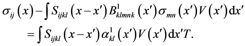
A similar equation may be written for the stress field σ(x) in the medium with the inclusions ([1,8]):
 (4)
(4)
Here  is an external stress field applied to the medium
 ,
,  ,
, 
 and
and
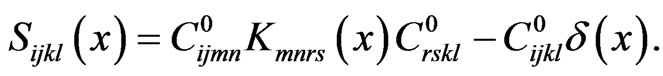 (5)
(5)
Note that the functions  and
and  in (2) and (5) behave as
  when
when , and therefore, the integral operators K and S in (1) and (4) are singular. Regularizations of these operators on continuous tensorfunctions with a finite support are indicated in [1,9]. Let
  be a smooth tensor-function which Fourier transform
  is bounded and tends to zero at infinity as
  or faster. In this case, the actions of the operators K and S on such a function are defined by the equations:
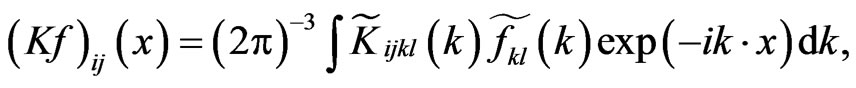 (6)
(6)
 (7)
(7)
The integrals in the right-hand sides of these equations exist as ordinary integrals. Here  and
and  are the Fourier transforms of the functions
  and
and . If the medium is isotropic, the functions
  and
and  take the forms:
 (8)
(8)
 , (9)
, (9)
 , (10)
where k is the vector parameter of the Fourier transform,  is the scalar product of the vectors k and x,
  and
and  are the Lame constants of the host medium,
 . (11)
 are the elements of the tensor basis introduced in [1] for presentation of fourth-rank tensors:
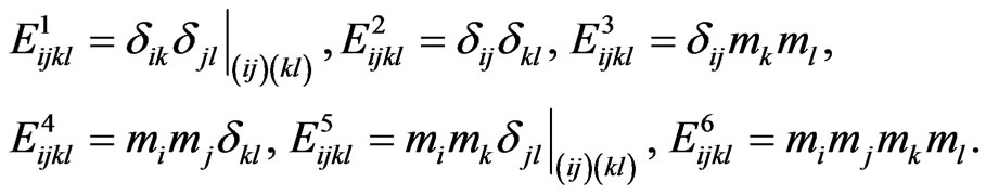 (12)
(12)
Because the strain  and stress
  tensors under the integrals in (1) and (4) are multiplied by the function
 , the elastic fields inside the inclusions (in the region V) are in fact the principal unknowns of the problem. The fields in the medium are reconstructed from the same Equations (1) and (4) if the fields inside the inclusions are known. Another important fact that follows from the structure of (1) and (4) is that for the numerical solution of this equation, any appropriate region
  that includes V may be considered. In particular, by the solution of the problem for an inclusion V of arbitrary shape one can consider a cuboid region
  that contains V (see Figure 1).
Unique solutions of (1) and (4) exist if the tensor of the elastic constants  and the inverse tensor
  do not degenerate inside V [9].
3. Numerical Solution of the Integral Equations (1) and (4)
3.1. Discretization of Equation (1) for Strains by the Gaussian Approximating Functions
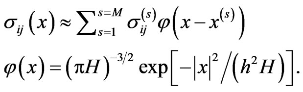
We consider Equation (1) for the elastic strains in a medium with heterogeneities and following to [6] find its solution in the form of the series:
 (13)
(13)
Here ,
,  are the nodes of a regular grid that covers a cuboid
  that contains the region V occupied by the inclusions, h is the distances between the neighbor nodes, M is the total number of the nodes in V,
  are unknown coefficients of the approximation. The parameter H has the order of 1
 . Substituting (13) into the integral in (1) leads to the following equation:
 (14)
(14)
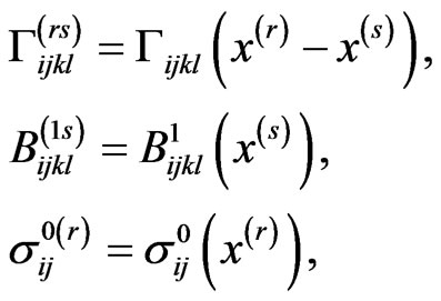
where , and the tensor
  has the form:
 (15)
(15)
Here, the definition (6) of the operator K and Equation (8) for  are used,
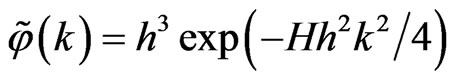 . (16)
Note that in (14),  if
if .
.
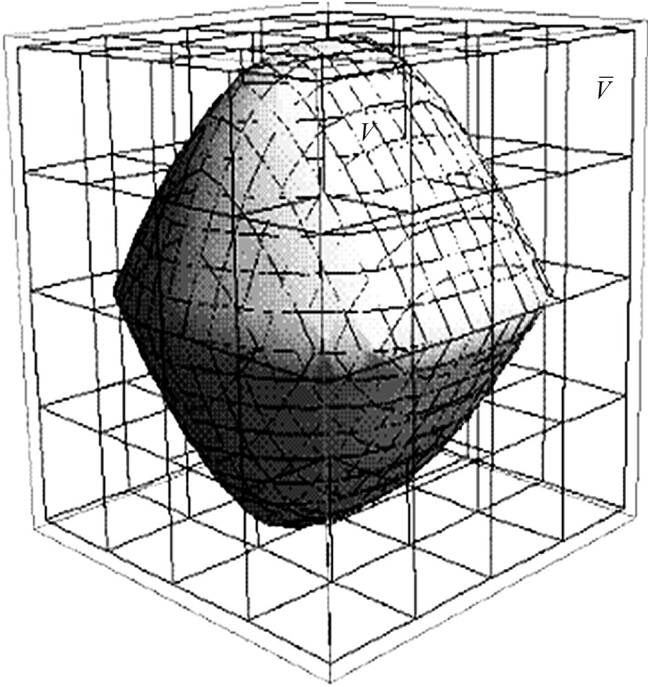
Figure 1. A cuboid  with an isolated inclusion V inside.
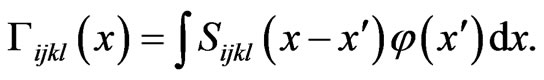
After introducing a spherical coordinate system in the k-space and integrating firstly over the unite sphere, and then, over the radius , the integral in the right hand side of (15) is calculated explicitly, and the tensor
  takes the form:
 (17)
(17)
 (18)
(18)
Here  are the elements of the tensor basis (12). The three scalar functions
 ,
,  ,
,  in (17) and (18) have the forms:
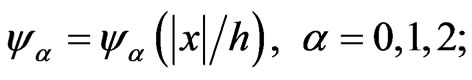 (19)
(19)
 (20)
(20)
 (21)
(21)
 (22)
(22)
Here  is the probability integral:
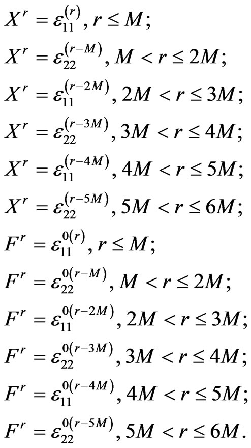
The system of linear algebraic equations for the unknowns  in (13) follows from (14) if the latter is satisfied at all the nodes (the Collocation Method). Note that if the nodes of the approximation (13) compose a cubic grid, the coefficients of the approximation
  coincide with the values of the strain field
  in the corresponding nodes (
 (see [6]). As a result, we obtain the system of linear algebraic equations for the coefficients
  in the form:
 (23)
(23)
 (24)
(24)
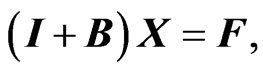
This system may be written in the canonical form as follows:
 (25)
(25)
where I is the unit matrix of the dimensions , and the vectors of the unknowns X and the right-hand side F are
 (26)
(26)
 (27)
(27)
Here  is the transposition operation.
The matrix B in (25) has the dimensions  and consists of 36 sub-matrices
  of the dimensions
 ,
,
 (28)
(28)
 (29)
(29)
 (30)
(30)
 (31)
(31)
 (32)
(32)
 (33)
(33)
 (34)
(34)
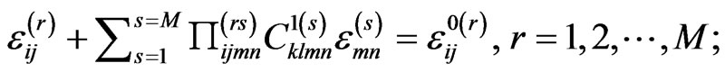
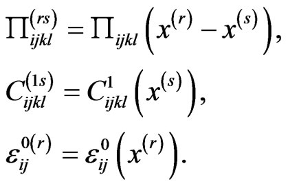
In these equations, ; summation from 1 to 3 with respect to repeating indices i, j is implied. These equations follow from (23) and (27). As it is seen from (19)-(22), the elements of the matrix B in (29)-(34) have simple analytical forms and are calculated fast.
3.2. Discretization of Equation (4) for Stresses by the Gaussian Approximating Functions
Let us consider (4) and find its solution in the form similar to (13):
 (35)
(35)
Substituting this approximation in (4) and using the Collocation Methods we obtain the following linear algebraic system for the coefficients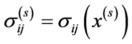 :
:
 (36)
(36)
 (37)
(37)
 (38)
(38)
The last integral is calculated similar to the integral in (15), and the tensor Γ(x) takes the following form:
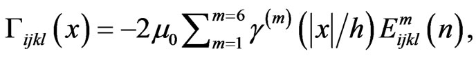 (39)
(39)
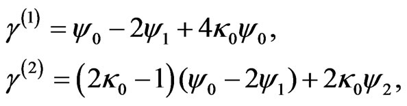 (40)
(40)
 (41)
(41)
Here the functions Φ0, Φ1, Φ2 and ,
,  ,
,  are defined in (18) and (19)-(22).
Similar to (23), the discretized Equation (36) may be presented in the canonical form (25). In this case, the vector of unknowns X is composed from the values of the stress tensor  at the nodes, the vector of the right hand side F consists of the components of the external stress field
  at the nodes similar to (26), (27). The matrices
  in (28) are defined in (29)-(34), where
  should be changed for
 , and
, and  for
for  .
.
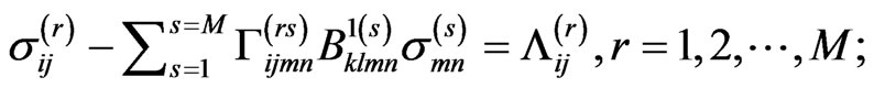
3.3. Numerical Solution of the System (25)
It follows from (17)-(22) and (29)-(34) that B in (25) is a non-sparse matrix which dimensions may be very large if high accuracy of the solution is required. For the solution of linear algebraic systems with such matrices, only iterative methods are efficient. For instance, if the Minimal Residue Method (see, e.g., [10]) is used, the n-th iteration  of the solution of (25) is calculated as follows:
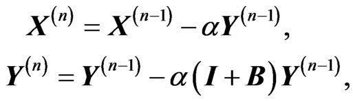 (42)
(42)
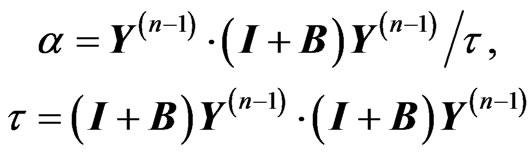 (43)
(43)
with the initial values X(0), Y(0) of the vectors X and Y
 . (44)
Thus, the vector  is to be multiplied by the matrix B at every step of the iteration process. For nonsparse matrices of large dimensions, calculation of such a product is an expensive computational operation. If, however, a regular grid of approximating nodes is used, the volume of calculations is reduced substantially. Let us consider the product BY in detail. For the matrix B that corresponds to (28)-(34), this product is a combination of the following sums:
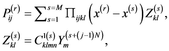 (45)
(45)
where the tensor  is defined in (17). For a regular node grid with a step h, the coordinates of every node
  can be presented in the form:
 (46)
(46)
 (47)
(47)
Here  are integers,
  ,
,  ,
,  are minimal values of the node coordinates in the cuboid V which sides are parallel to the axes
 ,
,  ,
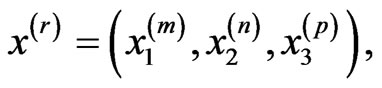
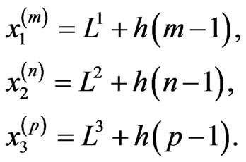
, . Thus, the position of every node may be defined by 3 integers (m, n, p). Connection between the one and three-index numerations of the nodes may be introduced by the equation:
 (48)
(48)
Here N1, N2, N3 is the number of the nodes along the corresponding sides of V, . In the threeindex numeration, the sum (45) is presented as follows:
 , (49)
 (50)
(50)
It is seen from the last equation that the object  has the Toeplitz structure: it depends on the differences of the indices:
 ,
,  and
and . As a result, the Fourier Transform Technique can be used for the calculation of the triple sums in (49), and therefore, of the matrix-vector products. Application of the FFT algorithms for calculation of these sums essentially accelerates the iterative process (42)-(44). In addition, one has to keep in the computer memory not all the matrices
  of the dimensions
  but only one column and one row of every such a matrix: the object that has the dimensions
  and is calculated once for all the iteration process. The details of the FFT algorithm for the calculation of the matrix-vector products are described in [7,11].
4. Results of the Calculations
4.1. An Isolated Heterogeneous Inclusion in a Homogeneous Elastic Medium
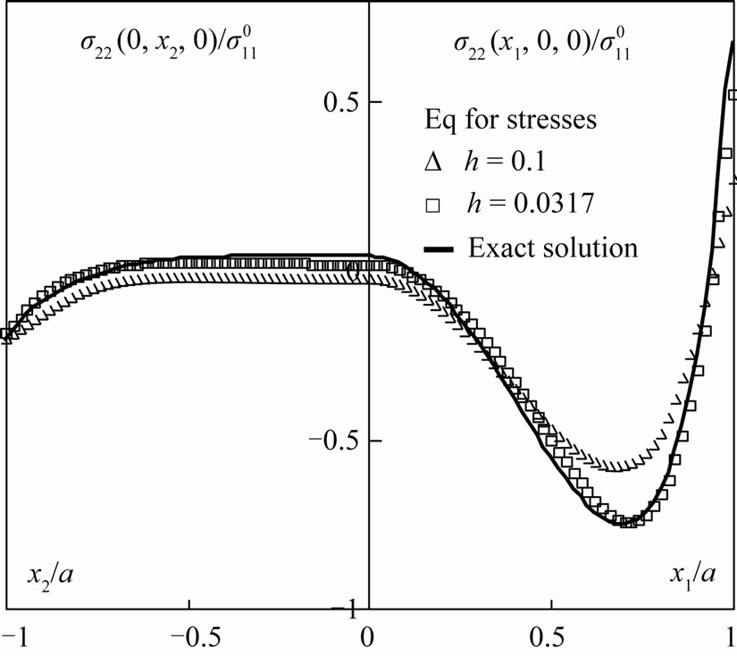
Let us apply the method to the calculation of elastic fields inside a spherical isotropic inclusion of a radius a with radially varying elastic properties. The elastic fields will be considered in a Cartesian coordinate system ( ) with the origin at the center of the inclusion. The medium is isotropic with the Young module E0 and the Poisson ratio
 . First, we consider an inclusion with parabolic change of the Young module
  along the radius:
 (51)
(51)
and constant Poisson ratio . The medium with the inclusion is subjected to a constant one-dimensional external stress field
  in the direction of the x1-axis,
  is a scalar. In this case, the Young module
  is a continuous function together with the components
  of the stress tensor. The distributions of the components
 ,
,  along the x1 and x2-axes are presented in Figures 2-3. While the functions
 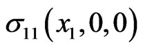 and
and 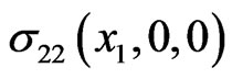 are on the right-hand sides in these figures, the functions
 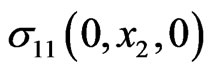 and
and 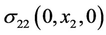 on their left-hand sides. The graphs in Figures 2-3 correspond to the numerical solution of Equation (4) for stresses inside the cube V:
 ,
, . The regular grids of approximating nodes with the steps
  (the total number of the nodes is
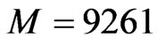 ), and
  (M = 262 144) were considered. The graphs in Figure 4 describe the distribution of the shear stress
  along the x1 and x3 axes if the medium is subjected to the external shear stress tensor
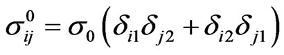 .
.
The bold lines in Figures 2-4 are exact distributions of the components of the elastic stress field obtained by the method presented in [8]. It is seen that for the grid step , the numerical solutions are practically coincide with the exact ones. The influence of the parameter H in (35) on the numerical results is not essential if
 , and
, and  is taken in the calculations.
The same problem was solved with the help of Equation (1) for strains. The medium was subjected to the
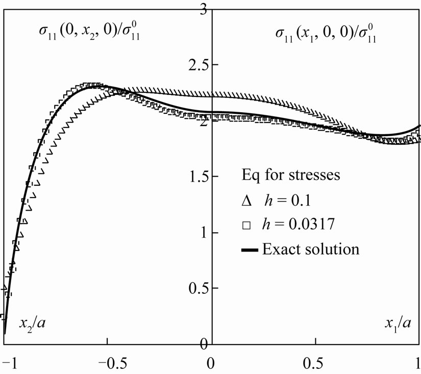
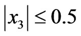
Figure 2. The dependence of the component σ11 of the stress field in a spherical inclusion with parabolic distribution of the elastic properties along the radius. The medium is subjected to a uniaxial stress field in the direction of the x1-axis.
 .
.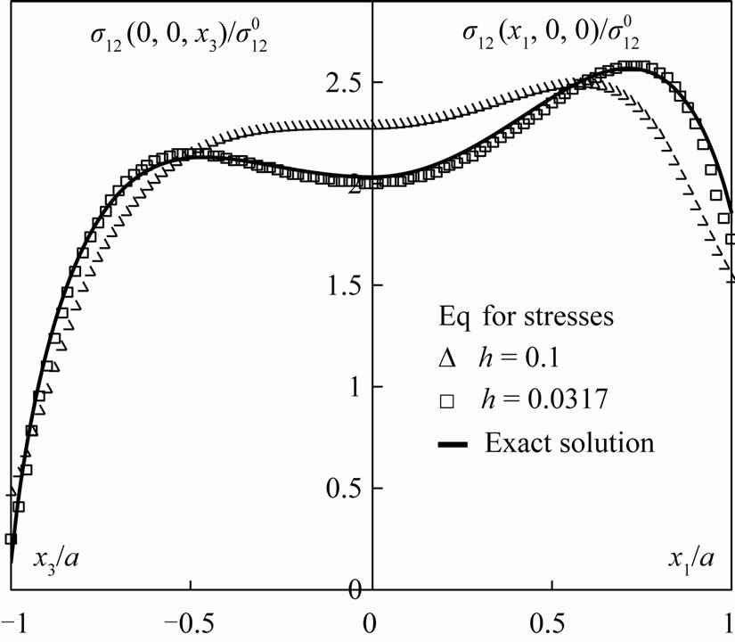
Figure 4. The same as in Figure 2 for the component , but the medium is subjected to a constant shear stress
 .
.
external strain field , where
  is a constant. The corresponding distributions of the components
  and
and  of the strain tensor inside the inclusion are in Figures 5-6. Figure 7 shows the distribution of the shear strain
  by application of the external shear strain tensor
 . The solid lines in these figures are exact distributions of the corresponding components of the strain tensor. It is seen that similar to the equation for stresses, the numerical solution coincides practically with the exact one for the step of the node grid
 . But the number of iterations in the process (42)-(44) turns out to be almost two times more than by the use of Equation (4) for stresses. This fact reflects general situation: the iteration process based on Equation (4) for stresses converges faster than the same process based on Equation (1) for strains if the inclusion is more rigid than the medium. In the opposite case, when the inclusion is softer than the medium, the iteration process based on the equation for strains converges faster than the same process based on the equation for stresses.
Note that if elastic moduli are not continuous on surfaces inside the inclusion or on the inclusion boundary, some components of the stress and strain tensors have jumps on these surfaces.
In this case, for accurate description of the elastic fields, the grid of the approximating nodes should be sufficiently fine. In the next example, we consider elastic fields in a spherical inclusion of the radius a that consists of a central kernel in the region  with the Young module
 , and a layer in the region
  with the Young module
 . The inclusion is embedded in a homogeneous medium with the Young module
 , Poisson ratios of the medium and the inclusion are the same
 . For the
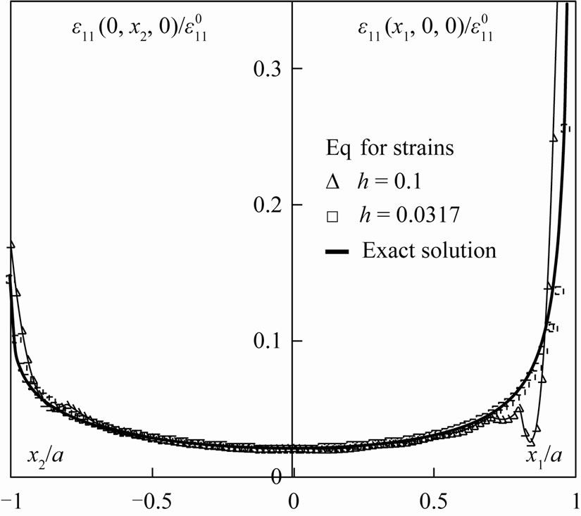
Figure 5. The dependence of the component ε11 of the strain field in a spherical inclusion with parabolic distribution of the elastic properties along the radius. The medium is subjected to a uniaxial strain field in the direction of the x1-axis.
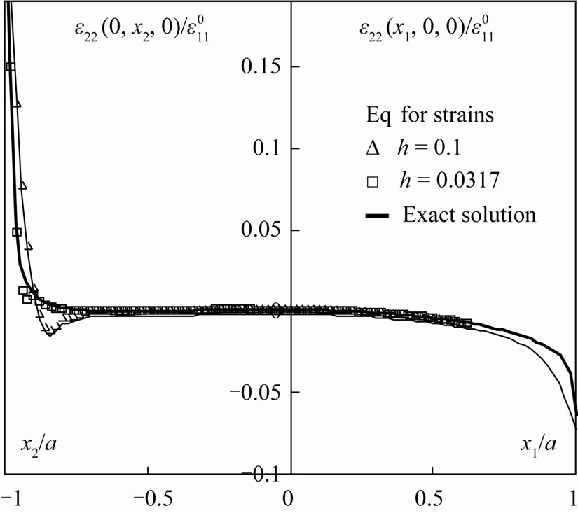
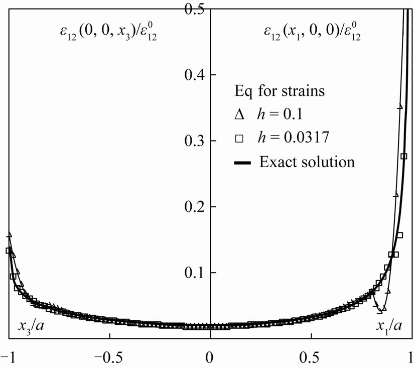
Figure 7. The same as in Figure 5 for the component , the medium is subjected to a constant shear strain
 .
.
uniaxial external strain field , the corresponding distributions of the components
  and
and  of the strain tensor inside the inclusion are presented in Figures 8-9. For the external shear strain field
 , the distribution of the component
  is in Figure 10. Equation (1) for strains and cubic node grids with the steps
 ,
,  (M = 68921) and
  (M = 8 120 601) were used for the construction of the graphs in Figures 8-10. The bold lines in these figures are exact solutions obtained by the method presented in [8]. It is seen from these figures that the numerical solutions tend to the exact one when the step h decreases.
The stress distributions in a layered spherical inclusion which Young moduli are more than the Young module of the medium are presented in Figures 11-13. In this case,  when
when  and
and 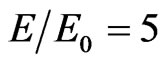 when 0.5<|x|/a≤1,
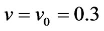 . The graphs in Figures 11-12 correspond to the uniaxial external stress field
 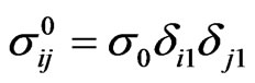 and in Figure 13 to the external shear stress field
 . For the numerical solutions, Equation (4) for stresses was used with the node grid steps
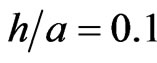 ,
,  , and
, and .
.
Figures 2-13 demonstrate convergence of the numerical solution to the exact distribution of the elastic fields inside the inclusions when step h decreases. The iterative scheme (42)-(44) converges for any finite values of the elastic constants of the inclusion and the matrix. The number of the iterations grows together with the contrast in the elastic properties of the matrix and the inclusion as well as with the number M of the approximating nodes. Note that for not very large contrast in the elastic properties of the medium and the inclusion, the well-known Conjugate Gradient Method (see, e.g., [10]) applied to the solution of (23) or (36) converges faster than the Minimal Residue Method (42)-(44). But for large contrasts in the properties, the Conjugate Gradient Method may diverge, meanwhile the Minimal Residue Method keeps converging.
4.2. Several Isolated Inclusions
Let a homogeneous medium contain three isolated spherical inclusions of equal radii  We assume that the centers of the inclusions are at the vertices
  of an equilateral triangle with the coordinates:
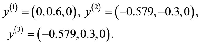 (53)
(53)
The numerical solution is constructed in the cuboid V that contains all these inclusions ( ,
, ,
, ) (Figure 14). The Young moduli of the medium and the inclusions are E0 and E, and
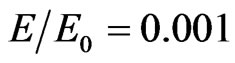 .
.
Figure 8. The dependence of the component ε11 of the elastic strain field inside a spherical inclusion with step-wise change of the elastic properties along the radius. The medium is subjected to a uniaxial strain field in the direction of the x1-axis.
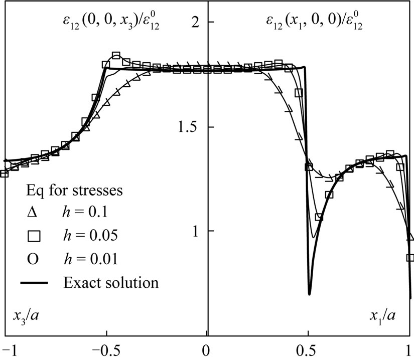
Figure 10. The same as in Figure 8 for the component , but the medium is subjected to a constant shear strain
 .
.
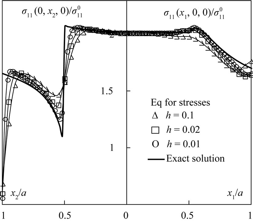
Figure 11. The dependence of the component σ11 of the elastic stress field inside a spherical inclusion with step-wise change of the elastic properties along the radius. The medium is subjected to a uniaxial stress field in the direction of the x1-axis.
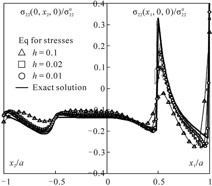
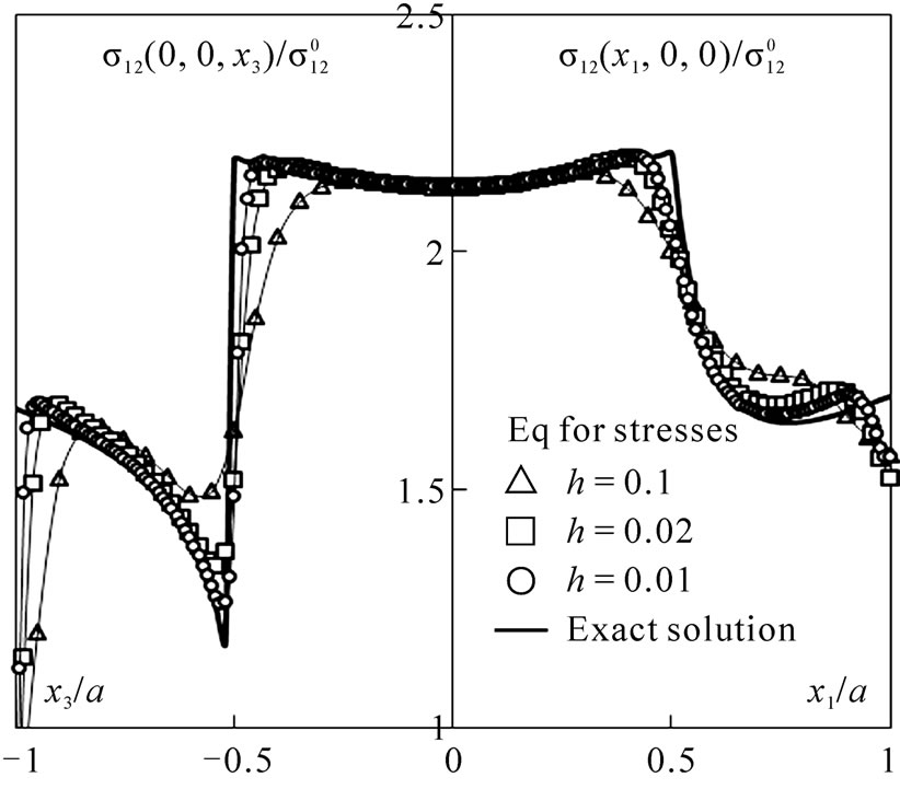
Figure 13. The same as in Figure 11 for the component , but the medium is subjected to a constant shear stress
 .
.
A cubic node grid with the step  (M = 1 030 301) and
  (M = 8 120 601) that covers the cuboid V was used in the calculations,
 . For the external uniaxial stress field
  acting along the x3-axis, the distribution of the component
 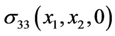 of the stress tensor in the plane
 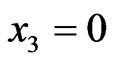 is presented in Figure 15. The distributions of the components
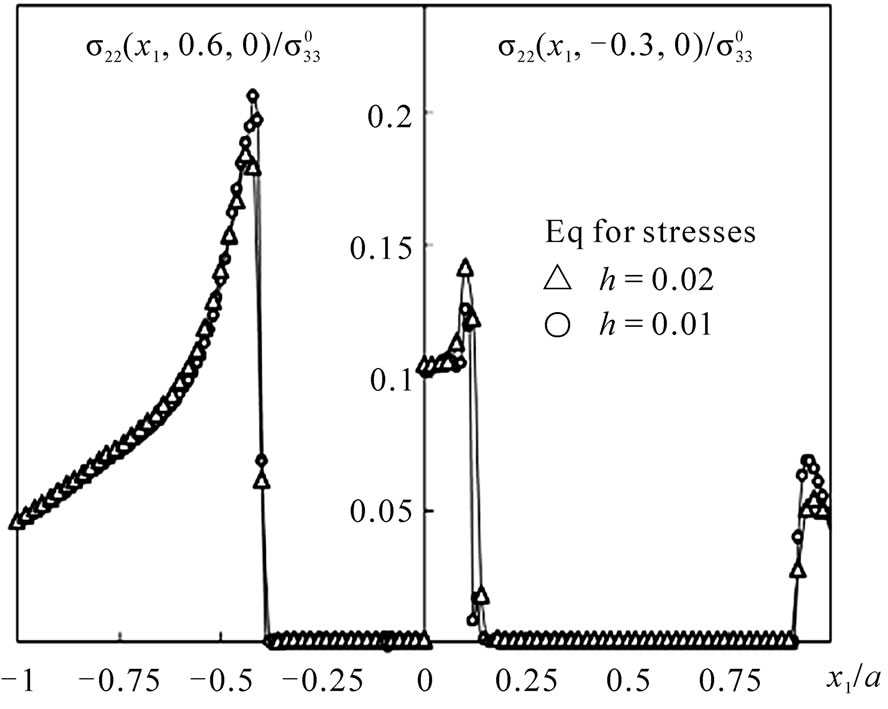
 ,
,  and
and  along the lines
 ,
,  and
and ,
,  that go through the centers of the inclusions are in Figures 16-18, correspondingly. For the solution, Equation (4) for stresses was used.
5. The Problem of Thermo-Elasticity
We consider a homogeneous elastic medium with several
Figure 14. A cuboid  with three spherical inclusions inside.
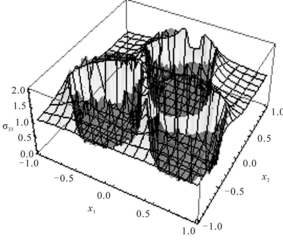
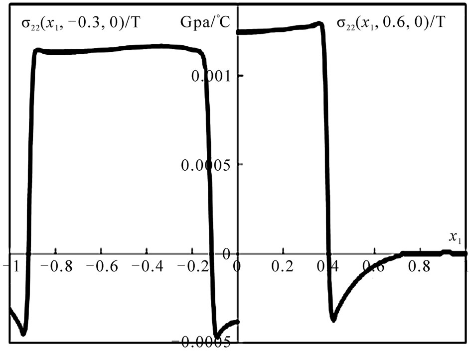
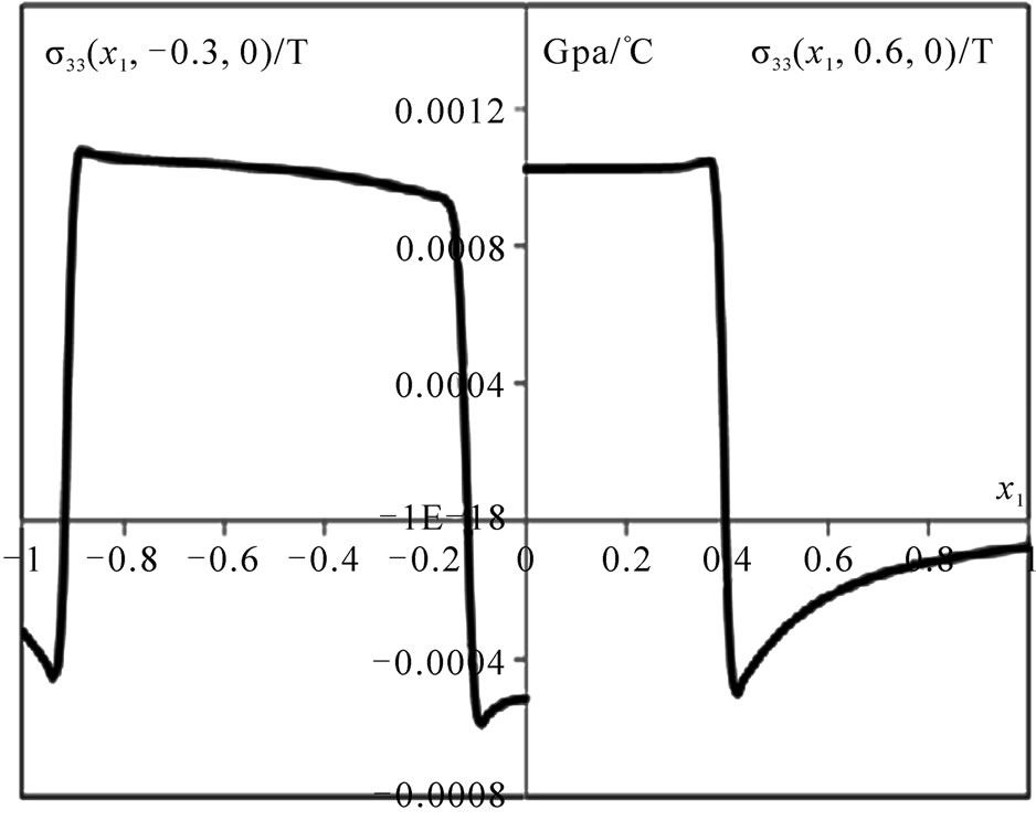
Figure 15. The distribution of the component σ33 of the stress field in the plane x3 = 0 inside the cuboid V; the medium is subjected to a uniaxial stress field in the direction of the x3-axis.
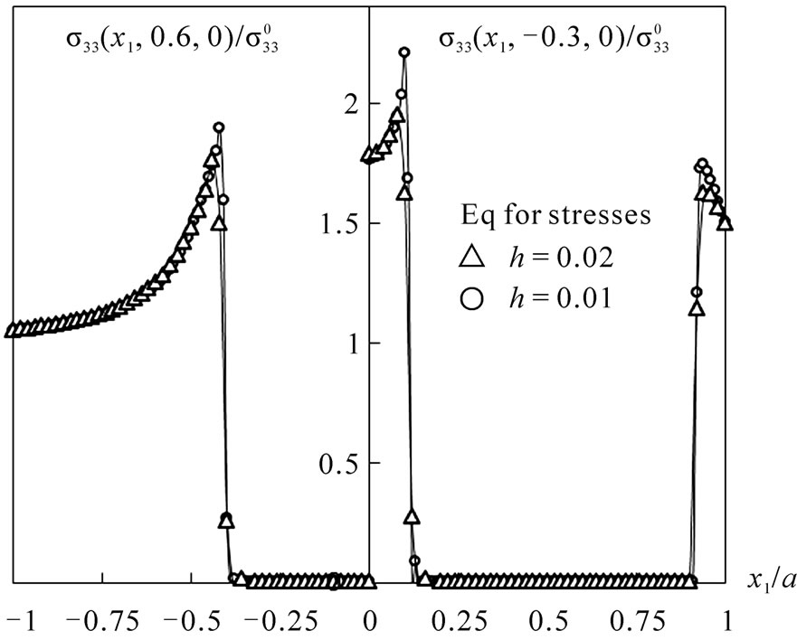
Figure 16. The distribution of the component σ33 of the stress field along the lines x2 = 0.6, x3 = 0 (left-hand side) and x2 = –0.3, x3 = 0 (right-hand side) that pass through the centers of the inclusions; the medium is subjected to a uniaxial stress field in the direction of the x3-axis.

heterogeneous inclusions that occupy regions Vk (k = 1,2, ). In addition to the elastic stiffness tensors
  and
and  of the inclusions and the host medium we introduce the second-rank tensors
  and
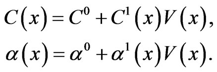
and  of thermal expansions of the corresponding materials. The tensors of the elastic stiffness and thermo-expansion of the medium with inclusions are represented in the forms:
 (53)
(53)
Here  is the characteristic function of the region occupied by the inclusions, the tensors
  and
and  are constant,
 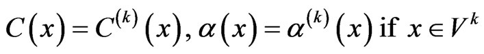 , and
, and ,
, if
if 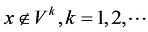 If the medium is subjected to an external stress field and a temperature field
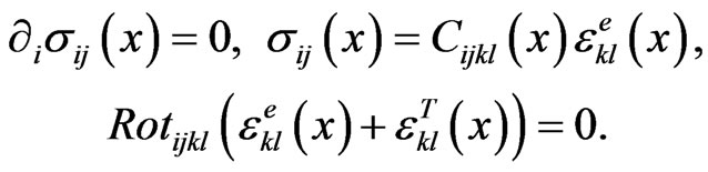
 , the stress tensor in the medium satisfies the following system of differential equations:
 (54)
(54)
Here  is the tensor of elastic deformation that defines the stress tensor σ according to Hooke’s law,
 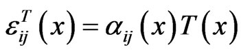 is the temperature deformation of the medium, and
 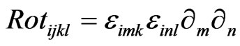 is the operator of incompatibility (
 is the Levi-Civita tensor). If we introduce an auxiliary tensor
  by the equation
 (55)
(55)
system (54) may be rewritten in the following form:
 (56)
(56)
 (57)
(57)
The system (56) may be interpreted as a system of differential equations for internal stresses in a homogeneous medium with the constant stiffness tensor  in the presence of dislocation moments of the density
 . The solution of (56) may be presented in the integral form (see [8,12]):
 (58)
(58)
Here  is an external stress field applied to the medium. The kernel
  of the integral operator in this equation coincides with the generalized function
  in (5), integration in (58) is spread over the entire medium. Substitution of the tensors
  and
and  from (57) and (53) into (58) yields
 (59)
(59)
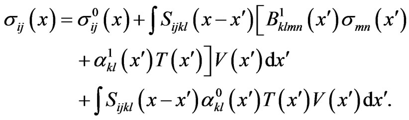
If , this equation coincides with Equation (4) for stresses in a medium with heterogeneities.
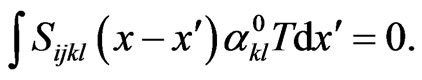
Let  be a constant temperature field, and for
 , the medium be free of the temperature stresses. In this case, the value of the last integral in (59) depends on the conditions at infinity. If deformation is not restricted at infinity, this integral is equal to zero (see [8]):
 (60)
(60)
Meanwhile, for the condition that the total deformation of the medium is equal to zero, we have
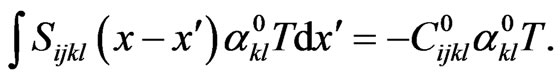 (61)
(61)
The right-hand side in this equation is the stress field in an infinite homogeneous medium with the properties ,
,  subjected to a constant temperature field T by the condition that the total deformation of the medium is zero.
In the absence of external stresses  and restrictions at infinity, (59) takes the form
 (62)
(62)
Approximation of the tensors  and
and  by the Gaussian functions similar to (35) and application of the Collocation Method lead to the following discretized form of this equation:
 (63)
(63)
 (64)
(64)
This system may be presented in the canonical form (25) which left-hand side coincides with the discretised form of Equation (4) for stresses, and the components of the vector F in its right-hand side are defined as follows:
 (65)
(65)
Because the objects  in (64) for
  have the Teoplitz properties, the FFT technique may be used for the calculation of the vector F.
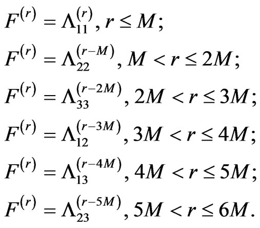
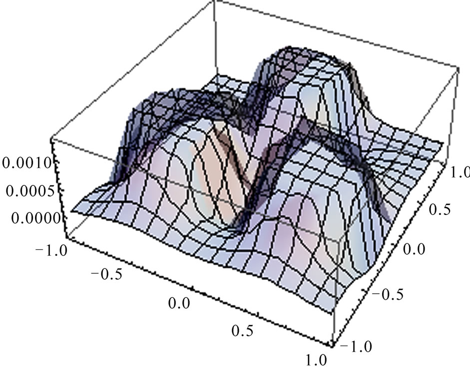
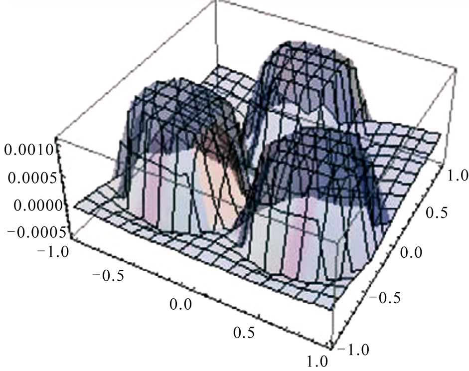
Distributions of temperature stresses in the medium with three spherical inclusions considered in Subsection 4.2 are presented in Figures 19-24. The Young’s module E0, Poisson ratio ν0, and the coefficient of thermo expansion
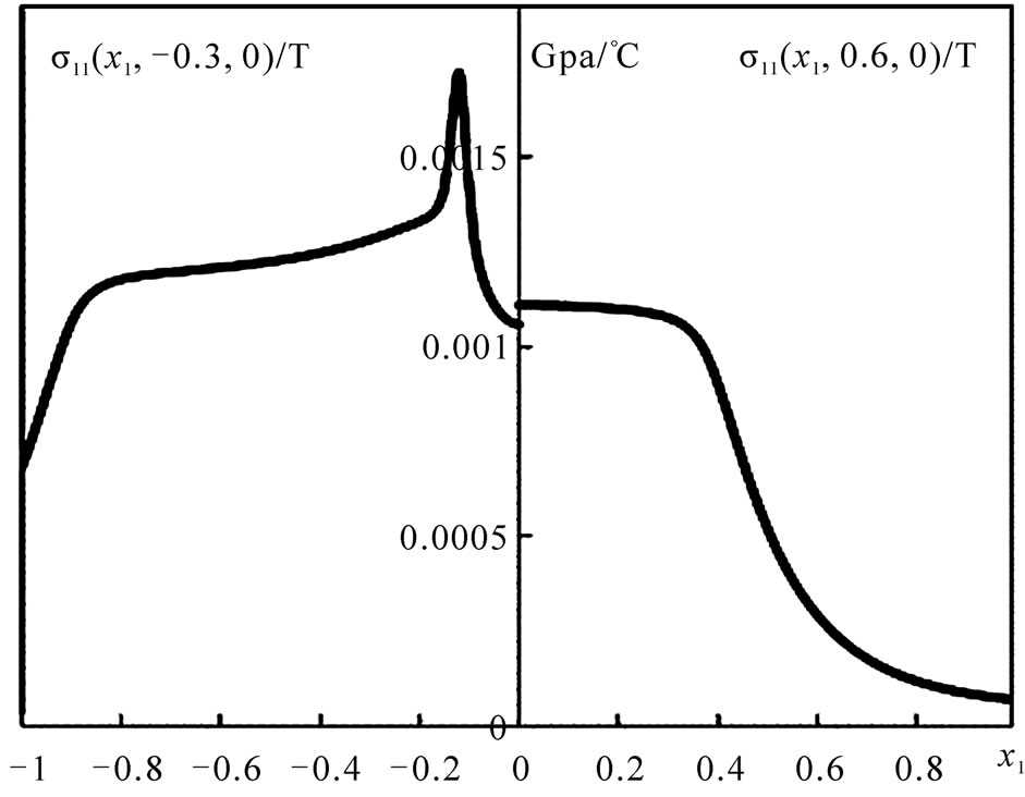
Figure 19. The distribution of the component σ11 of the thermo-stress tensor along the axes that go through of the centers of the inclusions shown in Figure 14.
Figure 20. The distribution of the component σ11 of the thermo-stress tensor in the plane x3 = 0 for the medium with three inclusions shown in Figure 14.
 of the host medium are taken as follows
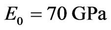 ,
,  , α0 = 23 × 10–6/˚C that corresponds to aluminum. The same parameters of the inclusions are
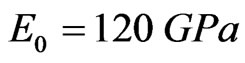 ,
,  , α0 = 9 × 10⁻⁶/˚C that corresponds to titanium. The solution of (64) was constructed in the cuboid
 ,
,  ,
, . The radii of the inclusions are taken
 . Note that the stress distribution does not depend on the absolute sizes of the inclusions. The distributions of the components
 ,
,  ,
,  of the stress tensor along the axis
  for
for 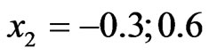 and
and  are shown in Figure 19, 21 and 23. The distributions of the same stresses in the plane
  are shown in Figures 20, 22 and 24. The calculations are performed for the step of the node grid
 ,
, .
.
Note that the integral equation for the stress field in an elasto-plastic heterogeneous medium follows from (57) and (58) if the temperature deformation T is changed for the plastic deformation . Because the plastic deformation is a non-linear function of stresses, the final equation will be non-linear with respect to the stress tensor. The conventional procedure of linearization of elasto-plastic problems is well known. The process of loading of the medium is divided into small intervals, and the problem is considered as linear in every such an interval. The same algorithm may be applied to the solution of the integral equation for the stresses in elasto-platic heterogeneous media.
6. Conclusions
An efficient numerical method for the solution of 3Dproblems of elasticity and thermo-elasticity for a medium with isolated heterogeneous inclusions is proposed. The method may be applied to the solution of other problems of mathematical physics that can be reduced to volume integral equations. In particular, in [13,14], the method was used for the solution of the problems of electromagnetic wave scattering on perfectly conducting screens and 3D-dielectric bodies.
The main difficulty in the numerical solution of 3Dintegral equations of mathematical physics is a large number of approximation functions (approximating nodes) that should be taken in order to achieve acceptable accuracy. In the present method, this difficulty is overcome by the following means. First, the Gaussian approximating functions allow us to obtain the elements of the matrix of the discretized problems in closed analytical forms and thus, to calculate them fast. Second, the use of regular node grids provides Toeplitz properties to the matrix of the discretized problem. As a result, the number of independent elements of this matrix is essentially reduced, and in addition, the FFT algorithms may be applied to calculating matrix-vector products with such matrices.
For some integral equations of mathematical physics or other types of approximating functions, the elements of the matrix of the discretized problem are not calculated explicitly but expressed via a finite number of standard one-dimensional integrals that can be tabulated (see [6,13]). So, in these cases, the matrices of the discretized problems are also calculated fast.
For regular node grids and any type of identical approximating functions centered at the nodes, the matrices of the discretized problems obtain the Toeplitz properties. Thus, in these cases, the possibility of exploiting FFT algorithms for the calculation of the matrix-vector products always exists.
There are various ways of improvement of the method. As it is shown in [6], the Gaussian functions multiplied with special polynomials increase the precision of the approximation. If such functions are used in the framework of the method, all the algorithms presented in this work will be the same, and only the form of the functions ,
,  , and
, and  in (19)-(22) will change.
Note that in the framework of the method, many parts of the problem may be calculated in parallel. For instance, the elements of the block-matrices in (29)-(34) and products of these matrices with vectors may be carried out independently, and at the same time. This is another advantage of the method and a source of accelerating of the computation process.
REFERENCES
- I. Kunin, “Elastic Media with Microstructure II,” Springer, Berlin, Toronto and New York, 1983.
- W. Chew, “Waves and Fields in Inhomogeneous Media,” Van Nostrand Reinhold, Amsterdam, 1990.
- A. Peterson, S. Ray and R. Mittra, “Computational Methods for Electromagnetics,” IEEE Press, New York, 1997. doi:10.1109/9780470544303
- C. Y. Dong, S. H. Lo and Y. K. Cheung, “Numerical Solution of 3d-Elastostatic Inclusion Problems Using the Volume Integral Equation Method,” Computer Methods in Applied Mechanics and Engineering, Vol. 192, No. 1-3, 2003, pp. 95-106. doi:10.1016/S0045-7825(02)00534-0
- C. Y. Dong, S. H. Lo and Y. K. Cheung, “Numerical Solution for Elastic Inclusion Problems by Domain Integral Equation with Integration by Means of Radial Basis Functions,” Engineering Analysis with Boundary Elements, Vol. 28, No. 6, 2004, pp. 623-632. doi:10.1016/j.enganabound.2003.06.001
- V. Maz’ya and G. Schmidt G, “Approximate Approximation,” American Mathematical Society, Mathematical Surveys and Monographs, Vol. 141, 2007, pp. 1-348.
- S. Kanaun, “Fast Calculation of Elastic Fields in A Homogeneous Medium with Isolated Heterogeneous Inclusions,” International Journal of Multiscale Computational Engineering, Vol. 7, No. 4, 2009, pp. 263-276. doi:10.1615/IntJMultCompEng.v7.i4.30
- S. Kanaun and V. Levin, “Self-Consistent Methods for Composites, Vol. 1: Static Problems (Solids Mechanics and Its Applications),” Springer, Dordecht, Vol. 148, 2008.
- S. Mikhlin, “Multidimensional Singular Integrals and Integral Equations,” Pergamon Press, Oxford & New York, 1965.
- W. H. Press, B. P. Flannery, S. A. Teukolsky and W. T. Vetterling, “Numerical Recipes in FORTRAN: The Art of Scientific Computing,” 2nd Edition, Cambridge University Press, New York, 1992.
- G. Golub and C. Van Loan, “Matrix Computations,” Johns Hopkins University Press, Baltimore, 1993.
- I. Kunin, “Methods of Tensor Analysis in the Theory of Dislocations,” US Department of Commerce, Clearinghouse for Federal Scientific Technology and Information, Springfield, VA 221151, 1965.
- S. Kanaun, “A Method for the Solution of the Diffraction Problem on Perfectly Conducting Screens,” Journal of Computational Physics, Vol. 176, No. 1, 2002, pp. 170- 190. doi:10.1006/jcph.2001.6974
- S. Kanaun, “Scattering of Monochromatic Electromagnetic Waves on 3D-Dielectric Bodies of Arbitrary Shapes,” Progress in Electromagnetics Research B, Vol. 21, No. 1, 2010, pp. 129-150.