International Journal of Astronomy and Astrophysics
Vol.09 No.01(2019), Article ID:90925,18 pages
10.4236/ijaa.2019.91003
Libration Points in the R3BP with a Triaxial Rigid Body as the Smaller Primary and a Variable Mass Infinitesimal Body
M. R. Hassan1, Sweta Kumari2, R. R. Thapa3, Md. Aminul Hassan4
1Department of Mathematics, S. M. College, T. M. Bhagalpur University, Bhagalpur, India
2T. M. Bhagalpur University, Bhagalpur, India
3Department of Mathematics, P. G. Campus, Tribhuvan University, Biratnagar, Nepal
4GTE, Bangalore, India

Copyright © 2019 by author(s) and Scientific Research Publishing Inc.
This work is licensed under the Creative Commons Attribution International License (CC BY 4.0).
http://creativecommons.org/licenses/by/4.0/


Received: November 8, 2018; Accepted: March 2, 2019; Published: March 5, 2019
ABSTRACT
The paper deals with the existence of the coplanar libration points in the restricted three-body problem when the smaller primary is a triaxial rigid body and the infinitesimal body is of variable mass. Following small parameter method, the coordinates of collinear libration points are established whereas the coordinates of triangular libration points are established by classical method. It is found that the mass reduction factor has small effect but triaxiality parameters of the smaller primary have great effects on the coordinates of the libration points.
Keywords:
Restricted Three-Body Problem, Jean’s Law, Space-Time Transformation, Triaxiality, Mass Reduction Factors, Libration Points

1. Introduction
Restricted three-body problem with variable mass has an important role in celestial mechanics. The phenomenon of isotropic radiation or absorption in stars was studied by the leading scientists to formulate the restricted three-body problem with variable mass. The two body problem with variable mass was studied by Jeans [1] regarding the evaluation of binary system. Meshcherskii [2] assumed that the mass is ejected isotropically from the two body system at very high velocities and is lost to the system. He examined the change in orbits, the variation in angular momentum and the energy of the system. Shrivastava and Ishwar [3] derived the equations of motion of the circular restricted three-body problem with variable mass with the assumption that the mass of the infinitesimal body varies with respect to time. Singh and Ishwar [4] showed the effect of perturbation due to oblateness on the existence and stability of the triangular libration points in the restricted three-body problem.
Das et al. [5] developed the equations of motion of elliptic restricted three-body problem with variable mass. Lukyanov [6] discussed the stability of libration points in the restricted three-body problem with variable mass. He has found that for any set of parameters, all the libration points in the problem (Collinear, Triangular) are stable with respect to the conditions considered by the Meshcherskii’s space-time transformation. El Shaboury [7] had established the equations of motion of elliptic restricted three-body problem (ER3BP) with variable mass with two triaxial rigid primaries. He has applied the Jeans law, Nechvili’s transformation and space-time transformation given by Meshcherskii in a special case.
Singh et al. [8] have discussed the non-linear stability of libration points in the restricted three-body problem with variable mass. They have found that in non-linear sense, collinear points are unstable for all mass ratios and the triangular points are stable in the range of linear stability except for three mass ratios depending upon the mass variation parameter governed by Jean’s law. Hassan et al. [9] studied the existence of libration points with variable mass in the R3BP when the smaller primary is an oblate spheroid. They found that Jacobi constant shows no effect in the position of libration points, but for , slight shifting of libration points is found due to oblateness only not due to the mass reduction factor .
In present work, we have established coordinates of five libration points in the R3BP with variable mass when smaller primary is a triaxial rigid body by small parameter method [10] and the method used by Hassan et al. [9] .
2. Equations of Motion
Let the two primaries of non-dimensional masses and be moving on the circular orbits about their centre of mass. In Figure 1, we consider a bary-centric coordinate system rotating relative to the inertial frame with angular velocity . The line joining the centers of and of the primaries is considered as the x-axis and a line lying on the plane of motion and perpendicular to the x-axis and through the centre of mass; as the y-axis and a line through the centre of mass and perpendicular to the plane of motion as the z-axis. Let and respectively be the coordinates of and and be the coordinates of the infinitesimal body of variable mass m at P.
The equation of motion of the infinitesimal body of variable mass m can be written as

Figure 1. Configuration of R3BP when smaller primary is triaxial.
(1)
the differential operators are given by the relations
(2)
where are the semi-axes of the triaxial rigid body, R is the dimensional distance between the centre of the primaries. Thus using Equation (2) in (1), we get
(3)
Choosing units of mass and distance in such way that and , then the equations of motion of the infinitesimal body in cartesian form can be written as:
(4)
where
(5)
(6)
By Jeans law, the variation of mass of the infinitesimal body is given by
(7)
where is a constant and the value of exponent for the stars of the main sequence (from Observational facts).
Let us introduce Meshcherskii’s space time transformations [2] as:
(8)
is the mass of the infinitesimal body when and is the pseudo time.
From Equation (7) and Equation (8), we get
(9)
where .
Differentiating with respect to t twice and using fourth equation of (8), we get
(10)
where dot represents differentiation with respect to real time t and prime represents the differentiation with respect to pseudotime .
Also,
Replacing the values of Equation (10) in Equation (4) to obtain
(11)
where
As the mass of the infinitesimal body is variable, so only the variational factors but not the non-variational factors should be taken into consideration in the equations of motion of the infinitesimal body. Thus to avoid the non-variational factors, we have
(12)
Thus the Equations (11) reduced to
(13)
where
(14)
(15)
The Jacobi integral in Meshcherskii’s space is
(16)
whereas the Jacobi integral in the rotating frame is
where
3. Libration Points
Since in the vicinity of the libration points (Lagrangian points), no translatory motion exists, only vibrational motion exists, hence velocity and acceleration components must vanish at these points i.e., .
Thus from Equations (15), we have
For solving the above equations in the rotating frame , we apply the inverse transformation in the above equations to get
(17)
4. Collinear Libration Points
As we know that all the three collinear libration points lie on the x-axis (the line joining the centre of the first and second primary) so and hence from Equation (2)
.
Thus from Equations (17), we have
(18)
Let be the first collinear libration point lying to the left of the second primary then
Thus from Equation (18),
(19)
As , so let where is a very small positive quantity.
From Equation (19)
(20)
(21)
(22)
Equation (22) is seven degree polynomial equation in , so there are seven values of . If we put then from Equation (22), we get
(23)
Here gives four roots of Equation (23) when but we know that so , so there must be some order relation between and
i.e., can be expressed as the order of i.e., where .
Thus the Equation (20) reduces to
(24)
As so can be expressed as
where are small parameters [10] , then
(25)
Using above quantities of Equation (25) and in Equation (24) and equating the coefficients of different powers of to zero, we get the values of small parameters as
(26)
where .
Therefore the first coordinate of the first libration point is given by
(27)
Here depends upon the mass parameter of the primaries, the small parameters , mass variation parameter , angular velocity and triaxiality parameters and . It is to be noted that each small parameters depends upon the preceeding small parameters and other parameters like etc. i.e., .
Thus from Equation (27), it is clear that in the classical case the coordinate of libration point depends upon the mass parameter only but under perturbation it depends upon the parameters as well as .
Let be the second collinear libration point between the two primaries and then .
Thus from Equation (18), we have
(28)
Since hence let , thus , is a very small quantity so it can be chosen as some order of .
In terms of , the Equation (28) can be written as
(29)
(30)
The Equation (30) is a seven degree polynomial equation in , so there are seven values of in Equation (30).
If we put in Equation (30), we get
(31)
Here also gives four roots of Equation (31) for , so as earlier case let
,
where are small parameters.
Putting the values of and in Equation (29) and equating the coefficients of different powers of , we get
where .
Similar to Equation (27), the coordinates of the Second libration point is given by
(32)
Let be the third libration point right to the First primary, then
Let then and .
Thus from Equation (18), we have
(33)
when , then Equation (33) reduced to
As in Equation (33) let , whereas are small parameters. Thus Equation (30) reduced to
By putting values of and in Equation (33) and equating the coefficients of different powers of , we get
and so on ,
where .
Similar to Equation (27), the coordinates of the third libration point is given by
(34)
5. Triangular Libration Points
For triangular libration points, and then from the system (17) we have
(35)
(36)
where from Equation (2)
(37)
Now Equation (35) Equation (36) gives
(38)
and Equation (35) Equation (36) gives
(39)
For the first approximation, suppose , then and from Equation (38) and Equation (39), we get
For better approximation let , then the above solutions can be written as
where .
From Equation (37) ,
(40)
Also from the first equation of (37), we have
From Equation (37), we have
.
So from Equation (38) and Equation (39), we get
Neglecting higher order terms and coupling terms of , we have
Thus
are the triangular libration points.
6. Discussions and Conclusion
We have studied the existence of coplanar libration points in the restricted three-body problem with variable mass and smaller primary as a triaxial rigid body as shown in Figure 1. By taking the mass ratio and the mass variation parameter as the fixed quantities, the variation of mass reduction factor of the infinitesimal body is taken into consideration and studied the effect of on the existence of coplanar libration points.
In Figure 2, the classical case has been discussed for in which all the five libration points exist. The triangular libration points and form equilateral triangle with the primaries. In Figure 3, taking perturbing parameters , then only three collinear libration points exist and no triangular points exist. The libration points and are located at the extreme points of the loop of the lamniscate shaped oval and this oval is again enveloped by a bigger loop. This development of loops is due to the non-zero values of triaxiality parameters and .

Figure 2. Locations of libration points for (classical case).

Figure 3. Locations of libration points for (perturbed case).
In Figure 4, two collinear libration points and exist when and , which contradicts theoretical evolution of the existence of the five libration points. In Figure 5, four coplanar points and exist for where and are collinear and and are non-collinear which don’t form the equilateral triangle with the primaries. The existence of and to the right of the origin is a contradiction to the theoretical evolution of the existence of libration points in the classical case of Figure 2 (Theory of Orbits [11] ).

Figure 4. Locations of libration points for (perturbed case).
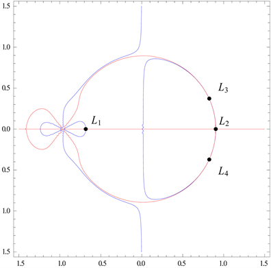
Figure 5. Locations of libration points for (perturbed case).
In Figure 6, when , all the five libration points exist with a difference. In Figure 6, the angular displacement of and relative to is more than that in Figure 5. Further when , angular displacement of and relative to is more in Figure 7 than that in Figure 6 and similar case is repeated in Figure 8 for . Thus due to the variational parameters and triaxiality parameters and , the location of triangular libration points and has been shifted from left to right and

Figure 6. Locations of libration points for (perturbed case).

Figure 7. Locations of libration points for (perturbed case).

Figure 8. Locations of libration points for (perturbed case).
the angular distances of and relative to increase with the decrease of . From the above discussions, we conclude that for and for , all the five libration points exist with an increase in angular displacement of and relative to with the decrease of and shifting of and from positive to negative side of the x-axis.
Conflicts of Interest
The authors declare no conflicts of interest regarding the publication of this paper.
Cite this paper
Hassan, M.R., Kumari, S., Thapa, R.R. and Hassan, Md.A. (2019) Libration Points in the R3BP with a Triaxial Rigid Body as the Smaller Primary and a Variable Mass Infinitesimal Body. International Journal of Astronomy and Astrophysics, 9, 21-38. https://doi.org/10.4236/ijaa.2019.91003
References
- 1. Jeans, J.H. (1928) Astronomy & Cosmogomy. Cambridge University Press, Cambridge.
- 2. Meshcherskii, L.V. (1949) Studies on the Mechanics of Bodies of Variable Mass. Gostekhizdat, Moscow.
- 3. Shrivastava, A.K. and Ishwar, B. (1983) Equations of Motion of the Restricted Three-Body Problem with Variable Mass. Celestial Mechanics and Dynamical Astronomy, 30, 323-328. https://doi.org/10.1007/BF01232197
- 4. Singh, J. and Ishwar, B. (1985) Effect of Perturbations on the Stability of Triangular Points in the Restricted Three-Body Problem with Variable Mass. Celestial Mechanics and Dynamical Astronomy, 35, 201-207. https://doi.org/10.1007/BF01227652
- 5. Das, R.K., Shrivastav, A.K. and Ishwar, B. (1988) Equations of Motion of Elliptic Restricted Three-Body Problem with Variable Mass. Celestial Mechanics and Dynamical Astronomy, 45, 387-393. https://doi.org/10.1007/BF01245759
- 6. Lukyanov, L.G. (1990) The Stability of the Libration Points in the Restricted Three-Body Problem with Variable Mass. Astronomical Journal, 67, 167-172.
- 7. El-Shaboury, S.M. (1990) Equations of Motion of Elliptically-Restricted Problem of a Body with Variable Mass and Two Triaxial Bodies. Astrophysics and Space Science, 174, 291-296. https://doi.org/10.1007/BF00642513
- 8. Singh, J. (2008) Non-Linear Stability of Libration Points in the Restricted Three-Body Problem with Variable Mass. Astrophysics and Space Science, 314, 281-289. https://doi.org/10.1007/s10509-008-9768-9
- 9. Hassan, M.R., Kumari, S. and Hassan, M.A. (2017) Existence of Libration Points in the R3BP with Variable Mass when the Smaller Is an Oblate Spheroid. International Journal of Astronomy and Astrophysics, 7, 45-61. https://doi.org/10.4236/ijaa.2017.72005
- 10. Volosov, V.M. (1972) Introductory Mathematics for Engineers. Mir Publishers, Moscow.
- 11. Szebehely, V. (1967) Theory of Orbits—The Restricted Problem of Three Bodies. Academic Press, New York and London.