Journal of Sensor Technology
Vol.1 No.3(2011), Article ID:7657,4 pages DOI:10.4236/jst.2011.13010
Direction of Arrival Estimation and Localization Using Acoustic Sensor Arrays
Department of Electrical and Computer Engineering, Illinois Institute of Technology, Chicago, USA
E-mail: erdal@ece.iit.edu
Received July 16, 2011; revised August 20, 2011; accepted September 6, 2011
Keywords: Sound Source Localization, Ultrasound, Acoustic Arrays, MEMS, Sound Imaging, Sound Tracking
Abstract
Sound source localization has numerous applications such as detection and localization of mechanical or structural failures in vehicles and buildings or bridges, security systems, collision avoidance, and robotic vision. The paper presents the design of an anechoic chamber, sensor arrays and an analysis of how the data acquired from the sensors could be used for sound source localization and object detection. An anechoic chamber is designed to create a clean environment which isolates the experiment from external noises and reverberation echoes. An FPGA based data acquisition system is developed for a flexible acoustic sensor array platform. Using this sensor platform, we investigate direction of arrival estimation and source localization experiments with different geometries and with different numbers of sensors. We further present a discussion of parameters that influence the sensitivity and accuracy of the results of these experiments.
1. Introduction
There is currently a significant amount of research and applications which use sound and ultrasound detection and analysis. Some of the research topics are multi-party telecommunications, hands-free acoustic human-machine interfaces, computer games, dictation systems, hearingaids, medical diagnostics, structural failure analysis of buildings or bridges, and mechanical failure analysis of machines such as vehicles or aircrafts, and robotic vision, navigation and automation [1-10]. In practice, there are a large number of issues encountered in the real world environment which make realistic application of the theory significantly more difficult [8,11-13]. This includes ambient sound and electrical noise, presence of wideband non-stationary source signals, presence of reverberation echoes, high frequency sources which require higher speed systems, and fluctuation of ambient temperature and humidity which affect the speed at which sound waves propagate.
This work emphasizes the design and development of sound and ultrasound localization systems. An introduction to commonly used terminology, concepts and mathematics is given. Real world application issues described above are addressed; this includes a presentation of how an anechoic chamber and acoustic arrays were used to create a controlled experimental setup in which noise, reverberation echoes, source distance and angles, number and geometry of sensors could be varied. Also presented is an FPGA based Micro-Electro-Mechanical Systems (MEMS) sensor platform for experimentation. In the following sections, we explain the sound localization techniques, introduce the proposed sensor platform and discuss the experimentation setups with the corresponding sound and ultrasound localization performance.
2. Background
Sound and ultrasound source localization is the process of determining the position of an acoustic source, such as a human speaker, a stereo system speaker, or an ultrasound transducer using two or more receivers or microphones. A similar but separate topic is direction of arrival estimation (DOAE) which only determines the direction of the sound source but not the distance to it [11]. Both localization and DOAE can be broken down into several types. One distinction that can be made is whether 2-dimensional (2D) source localization and DOAE or 3-dimensional (3D) localization and DOAE is being performed. This simply refers to only looking for a sound source in a plane, i.e. only horizontally or vertically, or in full 3D space. Another consideration of source localization is whether near-field or far-field modeling is being used [11,14]. Additionally, source localization can be categorized by the type of information used to perform the localization. These could be delays between the source’s transmit time and receivers’ pickup times, delays between only the receivers’ pickup times (known as time difference of arrival, TDOA), or power based localization. In this work, the first two sets of information are used as the power based methods are not sensitive enough for accurate estimations when using a passive system.
Localization and DOAE approaches can also be separated by the type of source signal being used, which could be continuous or pulse based, single amplitude or multiple amplitude, and single frequency or multiple frequency (in this work only single amplitude and single frequency source signals are used). Lastly, localization and DOAE can be separated by the type of TDOA and power based algorithms being used. For pulse based signals, the TDOA algorithm could be a threshold value detector which determines at which point a signal was transmitted or received. For continuous signals where phase is used the TDOA algorithm could be standard cross correlation, phase transform general cross correlation, or other algorithms [11-13,15].
In general, both localization and DOAE can be divided into three general steps: collecting data across multiple receivers and/or transmitters, finding the phase difference and/or time difference of arrival, and calculating the direction and possibly distance to the sound source. The two more complex steps are finding the phase difference/ TDOA and determining the angle/distance. As stated earlier finding the difference/TDOA depends on the type of algorithm used leading to a large number of approaches. Determining the angle and distance from the phase information depends on the interpretation of the collected data and depends on a large number of factors such as source signal type, the model being used, the number of receivers that are used, whether 2D or 3D estimation is being performed, and whether DOAE or localization is being performed.
3. Direction of Arrival Estimation
The geometry of 2D DOAE is illustrated in Figure 1. In this figure a source transmitter (Tx) is emitting a signal. This signal will then propagate through the air toward the two receivers (Rx1 and Rx2). As can be seen from the figure, since the two receivers are at different distances from the source the signal will reach them at different times, this is referred to as the TDOA marked as Τ. Based on this TDOA, the direction of the source with respect to the receivers can be estimated.
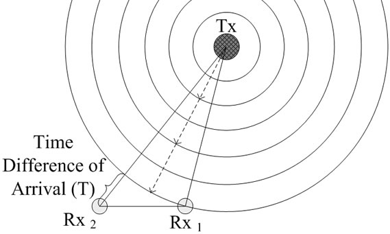
Figure 1. 2D DOAE geometry.
The estimation of the direction of the source can then be obtained through the use of the far-field model [11]. The far-field model assumes that the receivers are far enough away from the source as to allow the spherical wave propagation shown in Figure 1 to be approximated by planes. This model is shown in Figure 2.
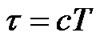
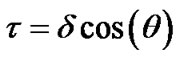
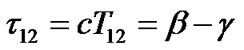
In this model the angle that the source makes to the plane connecting the two receivers is given by θ, the distance between the receivers is δ, and the distance corresponding to the TDOA is τ. The TDOA is the information that is directly obtained from the receivers and τ is given by Equation (1) below.
 (1)
(1)
where c is the speed of sound and T is the delay, in seconds between the two received signals. The inter-receiver distance is typically known since it can be set or measured by the designer or user. From this model it can be seen that the angle of the direction of the source to the receivers can be related to T and δ by Equation (2) given below.
 (2)
(2)
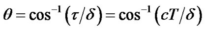
Thus Equation (3) below is the final equation which gives the direction of the source.
 (3)
(3)
4. Localization
2D localization can be performed with 3 receivers using only the TDOA information. The geometry for 2D local-
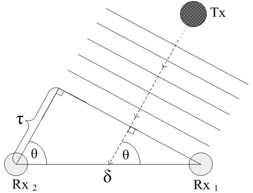
Figure 2. 2D DOAE far-field model.
ization using three receivers can be divided into two groups: one where the receivers are arranged in a line and the other where the receivers are arranged in a plane. The basic geometry and math with the receivers arranged in a line is shown in Figure 3 [11].
In this model, θ1, θ2 and θ3 are the angles from receivers 1, 2 and 3 to the source, respectively. α, β and γ are the distances from the source to receivers 1, 2 and 3, respectively. The distance between the receivers is δ. In this example, the two distances are made to be equal for simplicity. If they were different, the calculation would still work. The distances τ12 and τ13 are those corresponding to the TDOA between receivers 1 and 2, and between receivers 1 and 3, respectively, and are given by Equations (4) and (5).
 (4)
(4)
 (5)
(5)
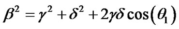
Using the law of cosines Equations (6) and (7) can be obtained to relate distances γ, α, β, δ and angle θ1.
 (6)
(6)
 (7)
(7)
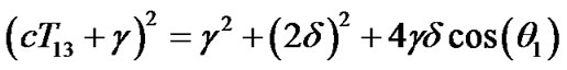
Equations (4) and (5) can then be substituted into Equations (6) and (7) to give Equations (8) and (9).
 (8)
(8)
 (9)
(9)
Equations (8) and (9) are two equations in two unknowns since the Τ12 and the Τ13 will be the collected data and δ as well as c are known quantities. Using Equations (8) and (9) the variables γ and θ1 can be solved for. Next Equations (4) and (5) can be used to solve for β and α. Now applying the cosine rule to triangle γ, δ, β gives angle θ2 and applying the cosine rule to triangle β, δ, α gives angles θ3. Thus, the distance and angle from each receiver can be obtained.
3D localization can be decomposed into two problems of 2D localizations as shown in Figure 4. Here three
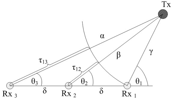
Figure 3. 2D localization geometry.

Figure 4. 3D localization geometry.
receivers in each plane are used in the same way that they were used for 2D localization, with both results using the same coordinate system centered at receiver 5. Since two planes are used all information about the source is obtained. Geometrically, this is the same as finding two circles, or semi-circles, the intersection of which is the location of the sound source.
5. Microphone Array Data Acquisition System
The MEMS Array acouStic Imaging (MASI) used in this work is a novel PC/FPGA based data acquisition system with an embedded MEMS based microphone array (see Figure 5). The data acquisition system is flexible, expandable, scalable, and has both logging and real-time signal processing capability. More specifically, the system can collect data from 52 omnidirectional microphones simultaneously at sampling rates up to 300 Ksps [10]. This data can be processed in real-time using the FPGA and then sent to a PC or alternatively the raw unprocessed data can be sent to a PC. The system to PC communications is performed through a gigabit Ethernet connection allowing high rates of transfer for the massive amount of data.
The system’s flexibility comes from the use of a central architecture called the Compact And Programmable daTa Acquisition Node (CAPTAN). This architecture was designed to be applicable to a variety of data acquisition problems and thus uses standardized and modular hardware, configware, and software [16]. Physically the sys-

Figure 5. MEMS Array acouStic Imaging (MASI).
tem can be separated into three parts namely the Node Processing and Control Board (NPCB), the Gigabit Ethernet Board (GEL), and the Acoustic MEMS Array (AMA). The NPCB is the backbone board that contains the FPGA which contains the system’s configware. The GEL board controls Ethernet communications. The MEMS board is the hardware which contains the microphones, amplifiers and analog to digital converters (ADC). Figures 5-6 illustrate the three hardware components that make up the system [16].
6. Anechoic Chamber and Sensor Array Test Stand
To create a controlled environment for acoustic experimentation a 52″ × 52″ × 27″ anechoic chamber was designed and built. The key features of the chamber are its ability to isolate the experiment inside the chamber from outside noise and to absorb sound inside the chamber to prevent multiple reflections (aka, reverberation). It should be noted that while the noise from outside of the chamber could be either reflected back outside or absorbed by the chamber, sound inside the chamber has to be absorbed by the surfaces of the chamber to prevent reflections. The material used for sound absorption was foam, however the chamber was designed in such a way that other materials with different acoustic absorption properties could be attached. The foam used was high density 2″ thick polyester-based polyurethane convoluted foam which is specifically designed for sound absorption. For ease of portability the chamber can be disassembled. Since the size and setup of the experiments which are to be performed are not known beforehand the chamber is designed to be modular allowing its size to be adjusted as necessary. Lastly, the chamber is designed to be easily opened and closed allowing the experimental setup to be quickly and effortlessly modified as necessary. Figure 7 shows the outside view of the assembled anechoic chamber.
In order to conduct a wide variety of acoustic and ultrasound experiments a sensor array test stand was designed and built. The key features of the test stand are its modularity and its configurability. These features allow
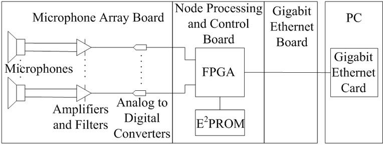
Figure 6. Functional block diagram of the microphone array data acquisition system.
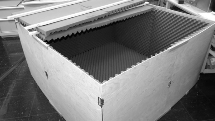
Figure 7. Anechoic chamber.
the user to vary the number, type, and arrangement of sensors while using the same test stand structure. Figure 8 below shows a picture of the sensor array test stand.
The sensor array test stand is made of a sensor bed and a stand. The sensor bed is 9.45″ × 11″, made from 2″ foam attached to a wooden backbone. Foam is used to reduce reflections and noise vibrations coupling. The sensor bed contains 25 sensor positions arranged in a 5 × 5 square layout. The backbone is attached to a rod stand using pinch clamps allowing the height and orientation of the sensors to be easily adjusted.
7. Sound Source Direction of Arrival Estimation Experiments
A variety of phase based sound source DOAE experiments were performed. The goal of the experiments was to determine the direction of the sound source with respect to the microphones. The direction of the sound source was calculated based on the recorded phase delay and the distance between the receiving microphones.
The first set of experiments involved the CAPTAN based microphone array data acquisition system and a transmitting speaker. The microphone array data acquisition system was mounted on vise base, the transmitting speaker was also mounted on a vise base. All 52 microphones of the system collected data at an acquisition rate of 300 Ksps each and two sets of microphones were used. The experiment was carried out in a laboratory room with
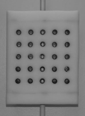

Figure 8. Sensor array test stand.
various random objects around the area of experimentation resulting in a high noise and a highly reflective environment.
The parameters varied in this experiment were the distance to the sound source, frequency of the sound source, the pairs of microphones used, and the angle between the sound source and the microphones. The overall geometry of the experiment is shown in Figure 9.
For the first test the distance between the receivers and transmitter was two feet and for the second test the distance was 5 inches. The sound source signal used was a continuous sine wave of frequencies 1 kHz and 2 kHz, generated by an arbitrary waveform generator. The distance between the inner set of receivers, as shown in Figure 10, was 0.39″, and the distance between the outer set of receivers, as shown in Figure 10, was 2.75″. The upper frequency was limited to 2 kHz to allow all microphones of the microphone array system to be used without aliasing. The maximum source signal frequency which could be used can be obtained from the spatial sampling theorem. This theorem states that for a given maximum temporal frequency in the source signal, there is a minimum spatial sampling, i.e. there is a maximum distance between the receivers used in the acquisition
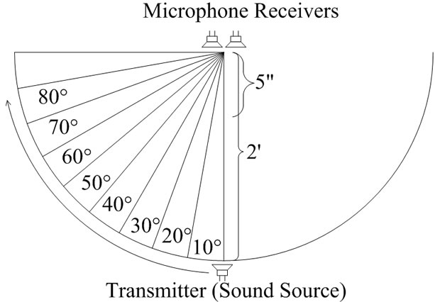
Figure 9. Sound source DOAE setup.
system. Specifically, this maximum distance is given by:
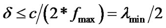 (10)
(10)
where δ is the maximum distance between the receivers, c is the speed of sound, fmax is the maximum frequency of the source signal, and λmin is minimum wavelength of the source signal.
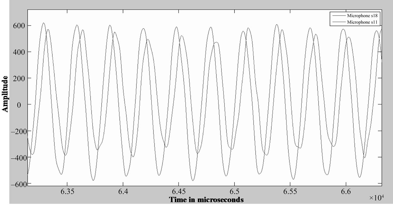
The sine wave pattern of the source signal collected by two of the microphones is shown in Figure 11. In this graph the phase difference between the data collected by the two MEM microphones can be clearly seen.
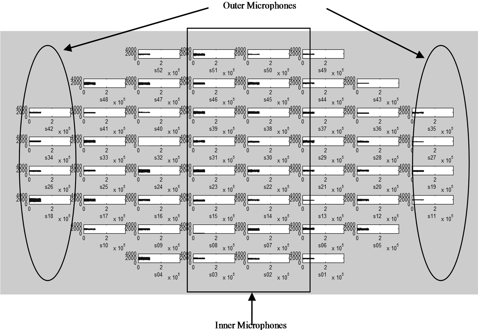
Figure 10 . Distribution of MEMS microphones.
7.1. DOAE Experiment Set 1 Using MEMs Array
The sets of microphones used for experimentation were the outer set and the central inner set (see Figure 10). For each set, the delay was obtained from each pair of opposing microphones; the results from each pair were then averaged to obtain the delay measurement for the set. The results of this set of experiments are shown in Tables 1-2. Here the angle of the sound source to the microphones is shown in the first column, the measurements for the two distances at two frequencies are shown in the second, third and fourth columns and the expected values are shown in the fifth column. The expected values for the two distances are presented as the same since the difference between them are less than 3% and are thus negligible. The results shown are those averaged for three trials at a frequency of 1 kHz and three trials at a frequency of 2 kHz. For visual inspection Figure 12 shows a results graph comparing the expected results versus those collected at 2 feet and at 5 inches for the 2 kHz source signal.
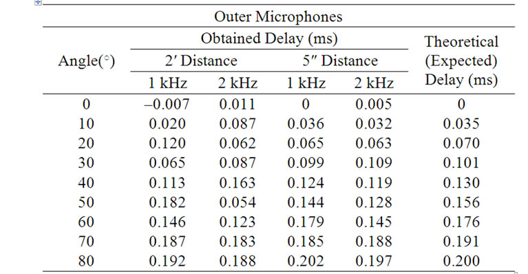
Table 1. Sound source DOAE experiment set 1, outer microphones results.
It can be seen from these results that phase based DOAE in a highly noisy and reverberant environment does not produce reliable results at larger distances independent of the frequency of the source signal or the distance between the receiving microphones. This can be seen from the mismatch between the collected data and the expected results, and also from the fact that the time
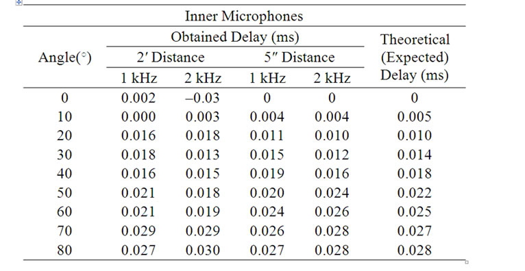
Table 2. Sound source DOAE experiment set 1, inner microphones results.
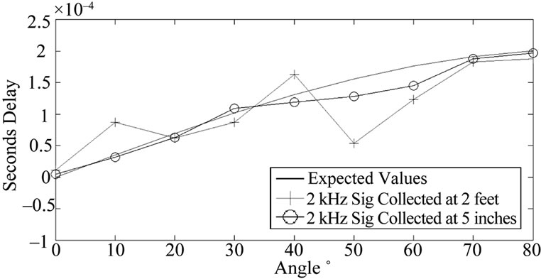
Figure 12. DOAE experiment set 1, expected results and 2 kHz results at 2′ and at 5″.
delays increase and decrease, instead of just increasing when the angle between the sound source and receiving microphones increases. It can also be seen that phase based DOAE works better at close distances where the power of the original signal is high compared to the power of the reflection based noise.
In summary, beamfield, frequency of the sensors, distance between the receiver and transmitter, and test environment contributing to the reverberation influence the accuracy of the measurements. Increasing the frequency of the transmitter or interrogation frequency allows higher sensitivity and narrower beamfield which is desirable for accurate readings. Main sources of reverberation are i) test environment, ii) receiver physical structure, and iii) prolonged signal from transmitters. In the following sections, we introduce practical steps to address each of these issues and improve the sound localization.
7.2. DOAE Experiment Set 2 Using Anechoic Chamber
In order to reduce the effect of reflection and ambient noise the second set of experiments were carried out inside the anechoic chamber. These experiments also used the CAPTAN based microphone array data acquisition system and a transmitting speaker. The experimental setup was the same as in the first set of experiments except for the use of the anechoic chamber. The results of this set of experiments are shown in Tables 3-4 below. For visual inspection Figure 13 shows a results graph comparing the expected results versus those collected at 2 feet and at 5 inches for the 2 kHz source signal.
From these results it can be seen that performing phase based sound source DOAE inside an acoustic chamber, which absorbs sound and thus reduces reflections, produces some improvement over performing sound source DOAE in a general room environment. This can be seen from the fact that the time delays increase as the angle between the sound source receiving microphones in
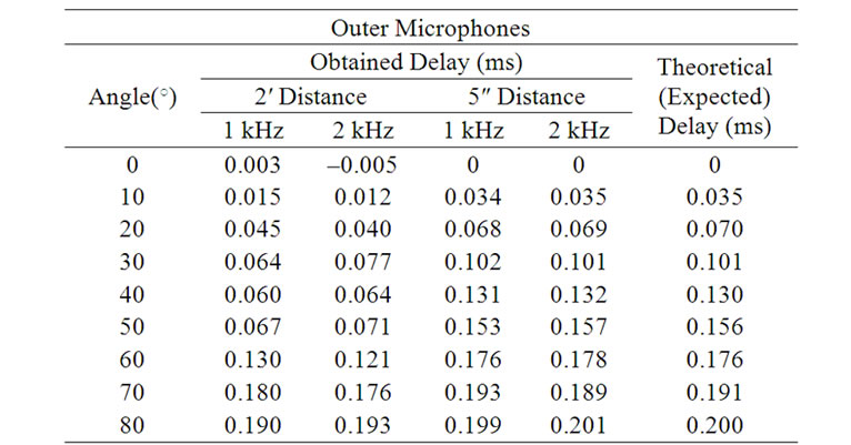
Table 3. Sound source DOAE experiment set 2, outer microphones results.
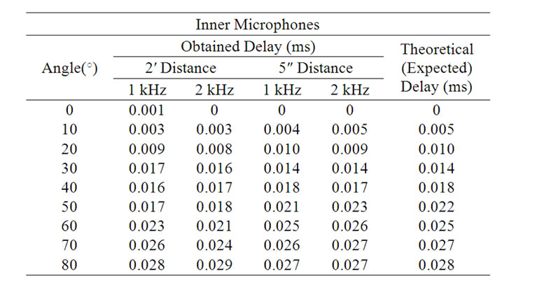
Table 4. Sound source DOAE experiment set 2, inner microphones results.
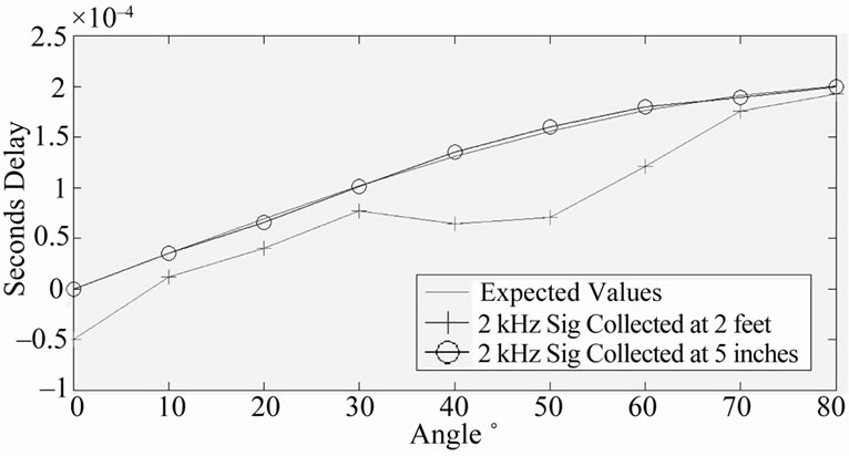
Figure 13. DOAE Experiment Set 2, Expected Results and 2 kHz results at 2′ and at 5″.
creases. However it can also be seen that the collected data still does not match the expected results thus there are still some reflections present in the environment. Again the frequency of the source signal and the distance between the receiving microphones affects the accuracy of the results.
7.3. DOAE Experiment Set 3 with Modified Receiver Physical Assembly
Since the surrounding surfaces inside the anechoic chamber absorb most of the sound, the reflections causing the distortions in this set of experiments came from the microphone array itself. In order to reduce the effect of the reflection, an alternate physical setup and acquisition system was used for the third set of experiments. The physical setup consisted of a vise with generic 60˚ beam angle microphone attached to each of the two arms of the vise through foam with nothing in between the vise arms, the distance between the microphones was increased to 6.3″. To comply with the spatial sampling theorem given in equation (10), the frequency of the source signals was changed to 700 Hz and 900 Hz to work with the greater distance between the receivers. The results of this set of experiments are shown in Table 5. For visual inspection, Figure 14 shows a results graph comparing the expected
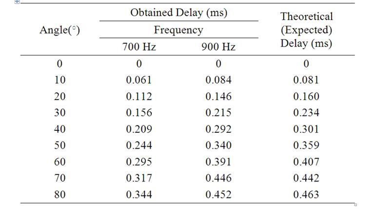
Table 5. Sound source DOAE experiment set 3 results.
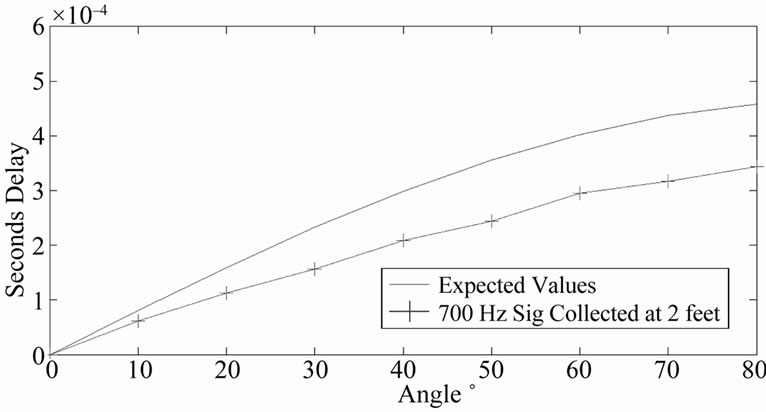
Figure 14. DOAE experiment Set 3, expected results and 700 Hz results at 2′.
results versus those collected at 2 feet for the 700 Hz source signal.
It can be observed that increasing the distance between the microphones and removing any reflective surfaces from in between the microphones significantly improves the accuracy of phase based DOAE even at larger distances. For the 900 Hz sound source signal the measured delays follow the correct pattern and are within a few percent of the expected time delays. For the 700 Hz sound source signal the measured delays also follow the correct pattern but the delays are a reduced version of the expected values, i.e. each measured delay is approximately 75% of the expected value. Thus the frequency of the sound source signal now has some effects on the measured time delay. This is again attributed to the remaining reflection in the environment.
7.4. DOAE Experiment Set 4 Using Shortened Transmission Signal
To further reduce the effects of reflection on the DOAE another set of experiments was performed. Here, the physical setup and the parameters varied were the same as for the third set of experiments except for the type of source signal used. This time instead of using a continuous sine wave for the source signal only a 20 cycle sine wave was transmitted. Then, when this sine pulse train wave was received, only the first pulse was used for phase comparison. This was expected to further reduce errors due to reflections since the first pulse should arrive before all reflections and thus its phase information should not be distorted. The results of this set of experiments are shown in Table 6 below. For visual inspection Figure 15 shows a results graph comparing the expected results versus those collected at 2 feet for the 700 Hz source signal.
From these results it can be observed that phase based DOAE which uses the phase information from only the first wave pulse provides accurate results even at larger distances and independent of the frequency of the source signal.
8. Ultrasound Localization Experiments
Higher accuracy measurements can be achieved by utilizing higher sound frequencies and narrower beamfields for both the transmitter and receiver. To demonstrate this, two types of ultrasound source localization experiments were performed. The first was a 2D ultrasound source localization experiment and the second was a 3D ultrasound source localization experiment. For both types of experiments localization was done based on the delays corresponding to the receiver to transmitter distances and

Table 6. Sound source DOAE experiment set 4 results.
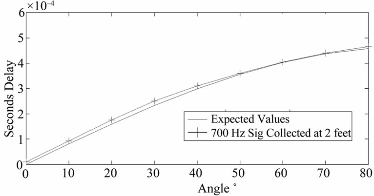
Figure 15. DOAE experiment set 4, expected results and 900 Hz results at 2′.
based on the time difference of arrival between the receivers.
Both of the experiments were carried out inside the anechoic chamber. The first experiment consisted of three generic 40 kHz ultrasound transducers which acted as receivers and one 40 kHz Measurement Specialties US40KT-01 omnidirectional ultrasound transmitter. The transmitter used a 20 cycle sine wave pulse train. The geometry and dimensions of the setup are shown in Figure 16.
In Figure 16, the transmitter is labeled Tx, and the receivers are labeled Rx1 through Rx3. The receivers were arranged in an equilateral triangle with a side length of 24″. The coordinates of each receiver and the transmitter, as well as the distances between each receiver and the transmitter are given by the figure above. Since this was a 2D experiment the transmitter and receivers were all at the same height or equivalently had a z coordinate of 0. The results of this set of experiments are shown in Table 7.
The second experiment consisted of six 40 kHz generic ultrasound transducers, five of which acted as receivers and one of which acted as a transmitter. The transmitter used a 20 cycle sine wave pulse train. The sensor array test stand as was used to hold the transmitter and receivers. The geometry and dimensions of the setup are shown in Figure 17. Here, the transmitter is labeled Tx, and the receivers are labeled Rx1 through Rx5. The receivers were arranged in a plus sign pattern. The results of this set of experiments are shown in Table 8.
Both sets of experiments produce accurate ultrasound
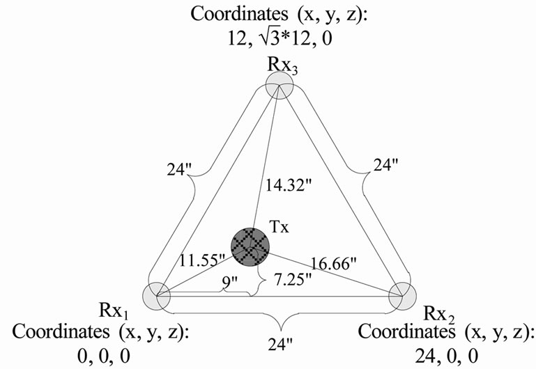
Figure 16. 2D Ultrasound localization setup.
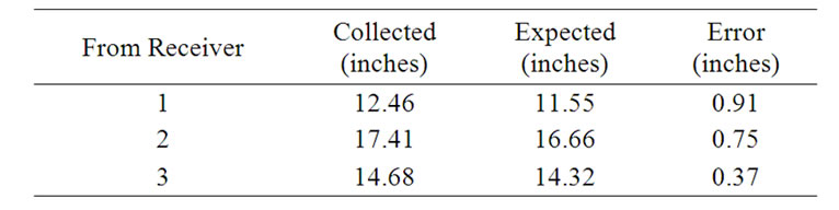
Table 7. Experimental results: 2D distances.

Figure 17. 3D, distances between the receivers and the transmitter.
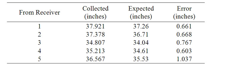
Table 8. Experimental results: 3D distances.
localization results and collected values are within a few percent of each other.
9. Conclusions
From the results, it can be seen that when certain restrictions such as a low reflection environment or the use of only the first part of a waveform are applied, phased based direction of arrival estimation can be used directly with reasonable accuracy. Parameters that affected the accuracy were the distance between the receivers and transmitter, the distance between the receivers, presence of reflective surfaces close to the receivers, and in some cases, the frequency of the source signal. Therefore, in this work, an anechoic chamber, improved physical assembly of the receiver end and a shortened transmission operation are implemented in order to improve the accuracy of the measurements.
The 40 kHz based ultrasound localization experiments showed even better accuracy and less susceptibility to noise and reflections. This was due to the application of the above stated restrictions to all the ultrasound experiments. The estimation techniques used in this work could be automated through the use of PCs, microcontrollers, or FPGAs for applications such as robotic auditory systems, voice based man machine interfacing and ultrasound beacon based object tracking.
10. References
[1] H. Alghassi, “Eye Array Sound Source Localization,” Doctoral Dissertation, University of British Columbia, Vancouver, 2008.
[2] J. Eckert, R. German and F. Dressler, “An Indoor Localization Framework for Four-Rotor Flying Robots Using Low-Power Sensor Nodes,” IEEE Transactions on Instrumentation and Measurement, Vol. 60, No. 2, 2011, pp. 336-344. doi:10.1109/TIM.2010.2085850
[3] S. Harput and A. Buzkurt, “Ultrasonic Phased Array Device for Acoustic Imaging in Air,” IEEE Sensors Journal, Vol. 8, No. 11, 2008, pp. 1755-1762. doi:10.1109/JSEN.2008.2004574
[4] S. J. Kim and B. K. Kim, “Accurate Hybrid Global Self-Localization Algorithm for Indoor Mobile Robots with Two-Dimensional Isotropic Ultrasonic Receivers,” IEEE Transactions on Instrumentation and Measurement, Vol. 99, 2011, pp.1-14,.
[5] J. R. Llata, E. G. Sarabia and J. P. Oria, “Three Dimensional Robotic Vision Using Ultrasonic Sensors,” Journal of Intelligent and Robotic Systems, Spring-Verlag, Berlin Heidelberg, Vol. 33, No. 3, 2002, pp. 267-284.
[6] Y. Ming, S. L. Hill and J. O. Gray, “Localization of Plane Reflectors Using a Wide-Beamwidth Ultrasound Transducer Arrangement,” IEEE Transactions on Instrumentation and Measurement, Vol. 46, No. 3, 1997, pp. 711-716. doi:10.1109/19.585438
[7] A. Nishitani, Y. Nishida and H. Mizoguch, “Omnidirectional Ultrasonic Location Sensor,” IEEE Sensors Conference, Irvine, October-November 2005, p. 4.
[8] J. C. Chen, K. Yao and R. D. Hudson, “Source Localization and Beamforming,” IEEE Signal Processing Magazine, Vol. 19, No. 2, 2002, pp. 30-39.
[9] C. C. Tsai, “A Localization System of a Mobile Robot by Fusing Dead-Reckoning, and Ultrasonic Measurements,” IEEE Transactions on Instrumentation and Measurement, Vol. 19, No. 5, 1998, pp. 1399-1404. doi:10.1109/19.746618
[10] M. Turqueti, J. Saniie and E. Oruklu, “Scalable Acoustic Imaging Platform Using MEMS Array,” EIT Electro/ Information Technology Conference, Normal, 20-22 May 2010, pp. 1-4.
[11] J. Benesty, J. Chen and Y. Huang, “Microphone Array Signal Processing,” Spring-Verlag, Berlin Heidelberg, 2008, pp. 211-215.
[12] M. Brandstein and D. Ward, “Microphone Arrays Signal Processing Techniques and Applications,” Spring-Verlag, Berlin Heidelberg, 2001.
[13] D. V. Rabinkin, R. J. Renomeron, J. C. French and J. L. Flanagan, “Estimation of Wavefront Arrival Delay Using the Cross-Power Spectrum Phase Technique,” 132nd Meeting of the Acoustic Society of America, Honolulu, 4 December 1996, pp. 1-10.
[14] I. McCowan, “Microphone Arrays: A Tutorial,” Doctoral Dissertation, Queensland University of Technology, Brisbane, 2001.
[15] J. M. Valin, F. Michaud, J. Rouat and D. L´etourneau, “Robust Sound Source Localization Using a Microphone Array on a Mobile Robot,” Proceedings of the 2003 IEEE/RSJ, International Conference on Intelligent Robots and Systems, Las Vegas, Vol. 2, 27-31 October 2003, pp. 1228-1233.
[16] M. Turqueti, R. Rivera, A. Prosser, J. Andresen and J. Chramowicz, “CAPTAN: A Hardware Architecture for Integrated Data Acquisition, Control and Analysis for Detector Development,” IEEE Nuclear Science Symposium Conference, Dresden, October 2008, pp. 3546-3552.