ABSTRACT

The problems of optimal control (OCPs) related to PDEs are a very active area of research. These problems deal with the processes of mechanical engineering, heat aeronautics, physics, hydro and gas dynamics, the physics of plasma and other real life problems. In this paper, we deal with a class of the constrained OCP for parabolic systems. It is converted to new unconstrained OCP by adding a penalty function to the cost functional. The existence solution of the considering system of parabolic optimal control problem (POCP) is introduced. In this way, the uniqueness theorem for the solving POCP is introduced. Therefore, a theorem for the sufficient differentiability conditions has been proved.

Keywords:

Constrained Optimal Control Problems, Necessary Optimality Conditions Parabolic System, Adjoint Problem, Exterior Penalty Function Method, Existence and Uniqueness Theorems

1. Introduction

Many researches in recent years have been devoted to the studies of optimal control problems for a distributed parameter system. Optimal control is widely applied in aerospace, physics, chemistry, biology, engineering, economics and other areas of science and has received considerable attention of researchers.

The optimal boundary control problem for parabolic systems is relevant in mathematical description of several physical processes including chemical reactions, semiconductor theory, nuclear reactor dynamics, population dynamics [1] and [2] . The partial differential equations involved in these problems include elliptic equations, parabolic equations and hyperbolic equations [3] [4] .

Optimization can be of constrained or unconstrained problems. The presence of constraints in a nonlinear programming creates more problems while finding the minimum as compared to unconstrained ones. Several situations can be identified depending on the effect of constraints on the objective function. The simplest situation is when the constraints do not have any influence on the minimum point. Here the constrained minimum of the problem is the same as the unconstrained minimum, i.e., the constraints do not have any influence on the objective function. For simple optimization problems it may be possible to determine, beforehand, whether or not the constraints have any influence on the minimum point. However, in most of the practical problems, it will be extremely difficult to identify it. Thus one has to proceed with general assumption that the constraints will have some influence on the optimum point. The minimum of a nonlinear programming problem will not be, in general, an extreme point of the feasible region and may not even be on the boundary. Also the problem may have local minima even if the corresponding unconstrained problem is not having local minima. Furthermore, none of the local minima may correspond to the global minimum of the unconstrained problem. All these characteristics are direct consequences of the introduction of constraints and hence we should to have general algorithms to overcome these kinds of minimization problems [5] [6] [7] [8] [9] .

The algorithms for minimization are iterative procedures that require starting values of the design variable x. If the objective function has several local minima, the initial choice of x determines which of these will be computed. There is no guaranteed way of finding the global optimal point. One suggested procedure is to make several computer runs using different starting points and pick the best Rao [10] . The majority of available methods are designed for unconstrained optimization, where no restrictions are placed on the de-sign variables. In these problems the minima, if they exist are stationary points (points where gradient vector of the objective function vanishes). There are also special algorithms for constrained optimization problems, but they are not easily accessible due to their complexity and specialization.

All of the many methods available for the solution of a constrained nonlinear programming problem can be classified into two broad categories, namely, the direct methods and the indirect methods approach. In the direct methods the constraints are handled in an explicit manner whereas in the most of the indirect methods, the constrained problem is solved as a sequence of unconstrained minimization problems or as a single unconstrained minimization problem. Here we are concerned on the indirect methods of solving constrained optimization problems. A large number of methods and their variations are available in the literature for solving constrained optimization problems using indirect methods. As is frequently the case with nonlinear problems, there is no single method that is clearly better than the others. Each method has its own strengths and weaknesses. The quest for a general method that works effectively for all types of problems continues. Sequential transformation methods are the oldest methods also known as Sequential Un-Constrained Minimization Techniques (SUMT) based upon the work of Fiacco and McCormick, 1968. They are still among the most popular ones for some cases of problems, although there are some modifications that are more often used. These methods help us to remove a set of complicating constraints of an optimization problem and give us a frame work to exploit any available methods for unconstrained optimization problems to solve, perhaps, approximately. [5] [6] [7] [8] [9] . However, this is not without a cost. In fact, this transforms the problem into a problem of non-smooth (in most cases) optimization which has to be solved iteratively. The sequential transformation method is also called the classical approach and is perhaps the simplest to implement. Basically, there are two alternative approaches. The first is called the exterior penalty function method (commonly called penalty method), in which a penalty term is added to the objective function for any violation of constraints. This method generates a sequence of infeasible points, hence its name, whose limit is an optimal solution to the original problem. The second method is called interior penalty function method (commonly called barrier method), in which a barrier term that prevents the points generated from leaving the feasible region is added to the objective function. The method generates a sequence of feasible points whose limit is an optimal solution to the original problem. Luenberger [11] illustrated that penalty and barrier function methods are procedures for approximating constrained optimization problems by unconstrained problems.

In the meanings of constrained conditions, these optimal control problems can be divided into control con-strained problems and state constrained problems. In each of the branches referred above, there are many excellent works and also many difficulties to be solved.

The rest of this paper is organized as follows. In Section 2, the proposed system of optimal control problem with respect to a parabolic equation is offered. Section 3 describes the analysis of existence and uniqueness of the solution of the POCP. In Section 4, the variation of the functional and its gradient is presented. Section 5 describes Lipschitz continuity of the gradient cost functional. Finally, conclusions are presented in Section 6.

2. Problem Statement

Consider the following POCP process be described in:

:

(1)

with the initial and the boundary conditions:

(2)

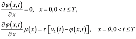(3)

where the solution of the problem (1-3) is, since, , the coefficient of convection is positive constant-sometimes is called coefficient of heat transfer. The admissible controls is a set defined as

Many physical and engineering settings have the mathematical model (1-3), in particular in hydrology, material sciences, heat transfer and transport problems [12] . In the case of heat transfer, the Robin condition physically is realized as follows. Let the surface of the rod be exposed to air or other fluid with temperature. Then is the temperature difference at between the rod and its surroundings. According to Newton’s law of cooling, the rate at which heat is transferred from the rod to the fluid is proportional to the difference in the temperature between the rod and the fluid, i.e.

(4)

The purpose is to find the optimal control that minimizes the following cost functional:

(5)

and

(6)

where are given positive numbers, is given function from , is given function from with is a fixed time. Penalty function methods are the most popular constraint handling methods among users. Two main branches of penalty method have been proposed in the literature: Exterior and Interior which is also called the barrier method. The basic idea in penalty method is to eliminate some or all constraints and add to the objective function a penalty term which prescribes a high cost to infeasible points. Associated with this method is a parameter, which determines the severity of penalty and as a consequence the extent to which the resulting unconstrained problem approximates the original constrained problem. We restrict attention to the polynomial order-even penalty function. The constrained optimal control problem (5-6) is converted to unconstrained optimal control pro- blem by adding a penalty function [13] to the cost functional (5), yielding the modified function:

(7)

where, , and, ,.

3. Well-Posedness of System

This section present the concept of the weak solution of the system (1-3) and the existence solution. Let a function of the weak solution of the problem, and satisfies the following integral, for all:

(8)

The weak solution of the direct problem exists and unique under the above conditions with respect to the given data [14] [15] . According to [12] , the solution of the optimal control problem can be defined as a solution of the minimization problem for the cost functional under condition (6), given by (5):

(9)

Theorem 1:

Under the above conditions, the optimal control problem has an optimal solution in.

Proof: when, the solution is a strict solution of systems (1-3) and (5-6), where satisfies the equation of functional,

. In parabolic problems and according to the theory of weak solution, can prove that the sequence weakly con-

verges to the function, so that the traces sequence of corresponding solutions of system (1-3) converges to the solution in, hence, when n→∞ then [16] . Therefore the func-

tional is weakly continuous on V, and the non-empty set of solutions for the minimization problem (5-6) [17] .

4. The Variation of the Functional and Its Gradient

The main objective here, the proof of Theorem 2 (found in tail of this section) which requires the following two lemmas; lemma 1 and lemma 2. Let the first variation of the cost functional of the cost functional (7) as follows:

(10)

therefore,

(11)

where

,

,

,

.

Therefore the function is the solution of the following system:

(12)

Lemma 1:

If the direct system (1-3) have the corresponding solution and is the solution of the adjoint parabolic problem [18] :

(13)

then the following integral identity holds for all elements and :

(14)

Proof: At with the condition in (13) to transform the left-hand side of (14) as follows:

At the boundary conditions in (13) and (14) for the functions and; we obtain (14). Corresponding to the inverse problem in system (1-3) and (5-6), the parabolic problem (13) define as an adjoint problem. By backward one of the Equation (13), the “final condition” at it is a well- posed initial boundary-value problem under a time reversal. The first variation of the cost functional obtain by using integral identity in (14) on the right-hand side of Equation (11):

(15)

Using the definition of the Fréchet-differential and the above the scalar product definition in V, transform the right-hand side of (15) need into the following expression:

(16)

Now we need to show that the last two terms on the right-hand side of (15) are of order, with.

Lemma 2:

If the parabolic problem (12) have the solution, , then the following inequality holds:

(17)

where is the norm of the function, is the norm of the function, and the constants, are defined as follows:

(18)

Proof:

Multiplying the Equation (12) by, then integrating the result on, ,.

We obtain energy identity after applying the initial and boundary conditions as the following:

(19)

We use the -inequality for the solution of the parabolic problem (19). Then for all we have:

(20)

Applying the Cauchy inequality to estimate the term:

By integrating the both sides of above inequality on, we obtain:

(21)

and use this estimate on the right-hand side of (20):

From (19) with above inequality, we obtain:

(22)

where and, we get bound (18) with for estimate (22):

Hence, the last integral (15) is bounded by and using Fréchet- differential definition at.

we obtain the following theorem:

Theorem 2:

The cost functional is Fréchet-differentiable in the considered problem hold, and Fréchet derivative at of can be defined by the solution of the adjoint problem (13) as follows:

(23)

5. The Continuity of Gradient Functional

In this section, by helping the gradient of cost functional we prove the Lipschitz continuity of. The minimization problem (9) need an estimation of the iteration parameter beginning with the initial iteration :

(24)

In many situation estimations of determine the parameter in various gradient methods is a difficult problem [19] . However, for arbitrary parameters, the parameter can be estimated via the Lipschitz constant in the case of Lipschitz continuity of the gradient as follows:

(25)

Lemma 3:

The functional is of Hölder class under the conditions of Theorem 2 and

(26)

where

(27)

where and for parameters, , the Lipschitz constant is defined in (22) as follows:

(28)

Proof: Let the following backward parabolic problem

(29)

has the solution. Therefore, using the initial and boundary conditions after multiplying both sides of Equation (29) by, and integrating on as in the proof of Lemma 2, we can get the following energy identity:

(30)

implies the following two inequalities:

(31)

and

(32)

Multiplying the first and the second inequality by and, correspondingly, summing up them, and then using the inequality (20) we obtain:

(33)

Computing of the second integral on the right-hand side of (26) by the same term. From the energy identity (30) we can obtain the following:

(34)

This, with the last estimate, concludes

(35)

where, using this in (27) and taking into account Lemma 2 we obtain (26) with the Lipschitz constant in (28).

6. Conclusion

In this paper, we studied a class of the constrained OCP for parabolic systems. The existence and uniqueness of the system is introduced. In this way, the uniqueness theorem for the solving POCP is introduced. Therefore, a theorem for the sufficient differentiability conditions has been proved. By using the exterior penalty function method, the constrained problem is converted to new unconstrained OCP. The common techniques of constructing the gradient of the cost functional using the solving of the adjoint problem is investigated.

Cite this paper

El-Sayed, M.A., Salama, M.M., Farag, M.H. and Al-Thobai- ti, F.B. (2017) The Cost Functional and Its Gradient in Optimal Boundary Control Pro- blem for Parabolic Systems. Open Journal of Optimization, 6, 26-37. https://doi.org/10.4236/ojop.2017.61003

References

- 1. Henry, D. (1981) Geometric Theory of Semi Linear Parabolic Equations. Lecture Notes in Mathematics, Vol. 840, Springer-Verlag, Berlin.
https://doi.org/10.1007/BFb0089647 - 2. Liu, H. and Yang, J. (2014) Optimal Control of Semi Linear Parabolic Systems with State Constraint. Journal of Mathematical Analysis and Applications, 417, 787-803.
https://doi.org/10.1016/j.jmaa.2014.03.070 - 3. Guliyev, H.F. and Jabbarova, K.H. (2011) On an Optimal Control Problem for Weakly Nonlinear Hyperbolic Equations. Acta Mathematica Hungarica, 131, 197-207.
https://doi.org/10.1007/s10474-011-0074-6 - 4. Tagiev, R.K. (2009) Optimal Coefficient Control in Parabolic Systems. Differential Equations, 45, 1526-1535.
https://doi.org/10.1134/S0012266109100164 - 5. Berhe, H.W. (2012) Penalty Function Methods Using Matrix Laboratory (MATLAB). African Journal of Mathematics and Computer Science Research, 5, 209-246.
- 6. De Sampaio, R.J.B., Wollmann, R.R.G., Yuan, J.Y. and Favaretto, F. (2014) Using Penalty in Mathematical Decomposition for Production-Planning to Accommodate Clearing Function Constraints of Capacity, Optimization and Control Techniques and Applications. Springer Proceedings in Mathematics & Statistics, 86, 137-152.
http://www.springer.com/series/10533 - 7. Farag, M.H., Nofal, T.A., El-Sayed, M.A. and Al-Baqmi, N.M. (2015) Computation of Optimal Controls for a Class of Distributed Parameter Systems. Journal of Computer and Mathematical Sci-ences, 6, 439-448.
- 8. Farag, M.H., Nofal, T.A., El-Sayed, M.A. and AL-Qarni, T.M. (2015) An Optimization Problem with Controls in the Coefficients of Parabolic Equations. British Journal of Mathematics & Computer Science, 6, 532-543.
- 9. Razzaghi, M. and Marzban, H.R. (2002) Optimal Control of Singular Systems via Piecewise Linear Polynomial Functions. Mathematical Methods in the Applied Sciences, 25, 399-408.
https://doi.org/10.1002/mma.297 - 10. Rao, S.S. (2009) Engineering Optimization: Theory and Practice. 4th Edition, John Wiley & Sons, Inc.
https://doi.org/10.1002/9780470549124 - 11. Luenberger, D.G. (1974) A Combined Penalty Function and Gradient Projection Method for Nonlinear Programming. Journal of Optimization Theory and Applications, 14, 477-495.
https://doi.org/10.1007/BF00932843 - 12. Hasanov, A. (2007) Simultaneous Determination of Source Terms in a Linear Parabolic Problem from the Final over Determination Weak Solution Approach. Journal of Mathematical Analysis and Application, 330, 766-779.
https://doi.org/10.1016/j.jmaa.2006.08.018 - 13. Aliay, M., Golalikhanib, M., Mohsen, M. and Zhuang, J. (2012) A Computational Study on Different Penalty Approaches for Solving Constrained Global Optimization Problems with the Electromagnetism-Like Method. Optimization, 63, 403-419.
https://doi.org/10.1080/02331934.2012.655691 - 14. Ladyzhenskaya, O.A. (1985) The Boundary Value Problems in Mathematical Physics. Springer-Verlag, New York.
https://doi.org/10.1007/978-1-4757-4317-3 - 15. Ladyzhenskaya, O.A., Solonnikov, V.A. and Ural’tseva, N.N. (1976) Linear and Quasilinear Parabolic Equations. Nauka, Moscow.
- 16. Mikhailov, V.P. (1983) Partial Differential Equations. Nauka, Moscow.
- 17. Gelashvili, K. (2011) The Existence of Optimal Control on the Basis of Weierstrass’s Theorem. Journal of Mathematical Sciences, 177, 373-382.
https://doi.org/10.1007/s10958-011-0463-y - 18. Lions, J.L. (1968) Contrôle optimal de systèmes gouvernés par des équations aux dérivées partielles. Dunod Gauthier-Villars, Paris.
- 19. Koppel, L.B. (1984) Introduction to Control Theory with Applications to Process Control. Prentice-Hall, Englewood Cliffs.