Open Journal of Energy Efficiency
Vol.05 No.02(2016), Article ID:67562,12 pages
10.4236/ojee.2016.52006
Conscious Use of the Virtual Sphere Modeling in the Simulation of Passive Night Cooling of Buildings
Marco Simonetti
Politecnico di Torino, Energy Department, Turin, Italy

Copyright © 2016 by author and Scientific Research Publishing Inc.
This work is licensed under the Creative Commons Attribution International License (CC BY).
http://creativecommons.org/licenses/by/4.0/


Received 8 May 2016; accepted 19 June 2016; published 22 June 2016
ABSTRACT
Night cooling of building is considered as a technology with a high potential of impact on air conditioning energy needs. Natural ventilation should be the first option for night cooling, for obvious reasons of energy savings. The evaluation of the capacity of the building to cool down its structures during night ventilation is of primary concern during preliminary design stage, even though night cooling with natural ventilation is among the most complex problem to be modelled in details. Some modelling options are available, assuming different simplifications in space and time. Among them, virtual sphere modelling has been proposed in the past as a quick way to perform dynamic simulation of the night cooling of buildings. In this paper, the theoretical origin of the virtual sphere model is recalled, underlining its limits in case of application to buoyancy driven night cooling of buildings. The limits can explain the disagreements of virtual sphere prediction with other methods reported in literature and may stimulate a more conscious application of the model and further improvements of the method.
Keywords:
Night Cooling of Buildings, Natural Ventilation, Virtual Sphere Modelling, CFD

1. Introduction
Night cooling is a building management strategy using low-temperature night air to cool the structural elements of the building itself, allowing them to store―without excessive overheating―the thermal loads released by occupants, electric devices, lighting equipment or transmitted through the envelope the day after. Conversely, it will remove the heat load stored the day before.
The night cooling technique has been widely studied in the past. In the 90s and first years of 2000, the most part of the published works focused on the potential of the night cooling technique, in some cases adding experimental results (see, among others: [1] - [4] ). Starting from the half of the last decade, a big effort has been devoted to the development of affordable and robust analytical/numerical models (for example [5] - [10] ). In those works, the authors tried to explain the most important mathematical dependencies and to develop numerical solutions. These tools should be able to answer to the question if and how much passive cooling is a good design choice, throughout the nearly 2000 to 4000 hours of a typical hot season, considering the most type of buildings and the settings of many different climatic and urbanization contests. However, a detailed transient analysis of some thousands hours of a couple thermo fluid dynamic problem, under a variety of profiles for boundary conditions, needs simplification assumptions or an extremely heavy full numeric approach. A letter by Pfafferot et al. [11] noted that “the building [dynamic] simulation provides accurate results, if the input parameters and boundary conditions are well known. However, user behavior results in energy and temperature variations which are of the same order of magnitude as the effect of different design decisions and operation strategies, respectively”.
More recently, some research papers had been published in which the authors developed parametric sensitivity analysis, in order to converge to a more conscious use of the numerical models (for example [11] - [15] ).
During the application of virtual sphere to a case of nocturnal natural ventilation [16] , some evident disagreement among CFD modelling, lumped parameter modelling and virtual sphere modelling emerged. In particular, the results of virtual sphere modelling were significantly different in terms of natural ventilation air flow rate and enthalpy flow rate.
The aim of this work is to analyse the theoretical origin of the virtual sphere model and to underline its limits in the specific application of buoyancy-driven night cooling of buildings, by considering the assumptions of the method and their role in the governing equation of natural night cooling.
2. Description of the Night Cooling
Natural nocturnal cooling of buildings can be considered physical problem of transient non-isothermal conjugated heat transfer, coupled with buoyancy and wind driven airflow. The main part of the phenomenon happens when the enclosed structures of the buildings are connected to an outdoor air flow, characterized by a temperature lower than the one of the structures themselves. Typically, windows are opened at night, outdoor air flows into the buildings in a cross ventilation pattern, cools down the structures and it is exhausted through vertical elements, such as stack, staircase and dwells.
A detailed analytical solution of the general problem is not available.
A complete suite of equations for the general case will include [17] - [19] :
the Navier-Stokes set for air (mass, momentum and energy conservation for a continuum fluid),
heat equation for building structures,
radiative heat transfer equation.
All these equations are coupled by the indoor air temperature (even if it is common that radiative heat transfer modelling for indoor environment considers the air perfectly transparent and not active in radiative heat transfer).
If the model of night cooling covers a time interval longer than one day, variable boundary conditions (outdoor environment) and intermittent and variable sources (internal loads) are to be considered. Further on, if the building is not in a free-running mode, i.e. if air conditioning is present, the model should take into account the plants and their control logics, for their role during the daily charging phase.
The air flow is induced by convection on the structural elements surfaces, but it is limited and strongly affected by the general building configuration, with the consequence that air velocity on the structure surfaces, the temperature of the solid and the average air temperature, are generally different from those of a similar free transient convection problem set in a free field condition.
During night cooling, in average, the indoor convection cooling is a natural, not forced, one. Let us virtually consider to expose the internal heat capacity of the building to the outdoor environment (Figure 1). The main difference with a natural cooling of the building structures, if virtually exposed outside of the building, would be that the real indoor air temperature is different from the free field one and it is coupled with the cooling of the building structures.
The air flow rate controls this temperature, and, as long as the ventilation is a buoyancy driven one, the air

Figure 1. Indoor vs. free-field set for cooling of building structures.
flow rate is a function of the indoor-outdoor difference of air temperatures. The standard set of lumped parameter modelling for natural ventilation has been reviewed in the past by Linden [20] .
Focusing on the heat transfer from the building masses to the air, the passive cooling can be considered a case of natural convection, even if the average airflow follows a path through the room, different from that followed in a free field case, due to natural forces and to the layout of the building. By the similarity theory methods, it is shown that for the convection problems the determining parameters are the numbers Gr, Pr and the complex:

often referred to as Richardson number (Ri),
where:
Gr = Grashof number = 
with
g = gravity acceleration [m/s2],
β = coefficient of thermal expansion for air (after Boussinesq approach) [-],
L = characteristic length [m],
Tw = wall temperature [K],
T∞ = air temperature (non disturbed) [K],
ν = cinematic viscosity [m2/s],
and
Re = local Reynolds number = uL/ν,
with
u = air velocity [m/s],
L = characteristic length [m],
ν = cinematic viscosity [m2/s].
When , the natural convection is prevailing, while when
 , the forced one is prevailing. An intermediate region is called a mixed convection region [21] .
For example, in the typical case study that will be described later and had been already investigated by use of CFD in [22] and [16] , Richardson number, calculated on the characteristic length of the slab in the direction of the transversal section of the building, was nearly 182. This number identifies a case dominated by natural convection.
Hence, the natural airflow is expected to influence the equilibrium indoor air temperature, while convection heat transfer on the solid is driven by buoyancy. Since we are considering an enclosure, radiation plays the sole role of rebalancing heat among the solids facing each other in the room: walls, ceiling and pavement.
This general description accepts some exceptions:
at a local level in the room Gr/Re2 can be in the region of mixed or even forced convection, because local higher air velocities are possible: for example, close to an airing opening or to a narrow window;
in case of a strong temperature difference (higher than 15˚C - 20˚C) buoyancy flows in a closure can organise in vortex on the scale of the room dimensions, in the wise of a thermosiphon loop, and increases local heat transfer coefficients. These effects have been used as an explanation to the reported higher value of heat transfer coefficients in enclosure, in comparison to free field, by Khalifa [23] . It has to be said that Khalifa’s experiment did not consider the outdoor airflow rate, but a closed test room.
In case of night cooling, indoor air temperature is always higher than outdoor one, thus the cooling of the building structures is expected to be always less effective than a virtual cooling of the same structures exposed in free field condition.
In general, available models of night cooling can be divided in two main categories (Figure 2): the ones that simplifies spatial description of physics in order to perform a far less time-consuming all year simulation (the dynamic zonal models of buildings) and the ones that pays for a more detailed spatial description with a practical limit in simulation time (a CFD model would belong to this second category). A quicker way and a third category is, naturally, the ones that assume simplifications in space and time.
Hybrid model with zonal framework coupled to local CFD are currently available, as well.
3. Theory of Virtual Sphere Modelling
3.1. Solution of Heat Equation for Natural Convection in a Free Field (Heisler Charts)
The transient heat conduction can be mathematically described by a second-order, parabolic, partial-differential equation. When applied to regular geometries such as infinite cylinders, spheres, and planar walls of small thickness, the equation is simplified to a single spatial dimension.
Let us consider the case of the plain wall that is somehow similar to a building’s slabs and walls. Starting from the one dimension (x) heat conduction equation:
 , (1)
, (1)
a solution is possible in association with boundary condition of central axe symmetry [19]
 , (2)
, (2)
applying convective heat transfer at position x = L
 , (3)
, (3)
and initial condition at t = 0
 (4)
(4)
where:
T = local temperature of the wall on the 1D domain [K] (variable),
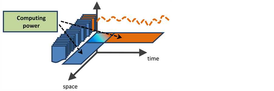
Figure 2. Schematics of models categories: computing power can be allocated for more detailed spatial description, paying in temporal step and extension, or can be used for a lumped modelling of space, simulated for a far longer period.
α = wall thermal diffusivity [m2/s] (constant),
h = mean convective heat transfer coefficient on the wall [W/(m2K)] (constant),
T∞ = convective air temperature [K] (constant).
Some following well known passages of nondimensionalization bring to the nondimensionalized problem:
 (5)
(5)
associated to the same previous boundary conditions, now described as:
 (6)
(6)
 (7)
(7)
and dimensionless initial condition
 (8)
(8)
where:
 dimensionless temperature,
 dimensionless distance from the center of symmetry,
 dimensionless heat transfer coefficient (Biot number),
Being k = slab and wall conductivity [W/(mK)] (constant),
 dimensionless time (Fourier number).
For this problem, a solution can be derived applying the separation of variable method. By doing so, the solution of the transient problem is derived in the form of an infinite series of term:
 (9)
(9)
where λ are eigenvalues of the associated characteristic equation.
Completely similar passages can be done for cylindrical and spherical coordinate, dealing with an infinite cylinder and a sphere.
Heisler [24] showed that for values of Fourier number Fo = (αt/L2) > 0.2, the infinite series solution can be approximated with a fair accuracy (an error within 1%) by the first term of the series. The approximated expressions for temperature distributions and heat flux had been plotted graphically and became widely known as Heisler Charts. The Heisler Charts consider solid having uniform initial temperature (Equation (4)) suddenly exposed to an environment at a different temperature (Equation (3)). They can be used to derive the temperature transient evolution of the solid centre and the 1D internal distribution, from centre to boundary, by calculating Fourier number (time scaling) and Biot Bi = hL/l number (ratio of convective heat transfer to conduction heat transfer rates) of the specific case, and reading ϴ value for the centre temperature on the charts.
3.2. The Virtual Sphere Model
The virtual sphere method was first proposed by Gao and Reid [25] , dealing with heat treatments in furnace. The idea was derived from the analysis of Heisler Charts for sphere, indefinite plate and cylinder, and consists of using only the sphere geometry to represent the work piece of any geometry. It has been observed that the Heisler charts for the three geometries are very similar to the one of a virtual sphere, if the radius of this sphere is chosen with a simple rule, added by the authors (Equation (12)). By this rule, the arbitrary shaped solid body could be converted into a virtual sphere, setting the characteristic length of the work piece as the radius of the sphere.
The idea was introduced in the field of indoor environment by Li and Yam [5] [6] . They suggested to lump up the mass elements into a virtual solid sphere with the radius determined from some significant dimensions of the mass (e.g. volume and surface area), consequently treating the mass elements as a single body. This approach requires less computation time, as large-scale heat transfer calculation of the mass elements is avoided. After the authors, the method could not provide accurate results, but is able to provide some guideline for the building services engineer, to evaluate how much thermal mass should be used in a particular design and what are the effects of various geometry designs of the internal thermal mass. This model has been cited several times in literature, directly and indirectly.
Once a virtual sphere model is defined, heat equation on the new domain can be solved with any methods.
Here we focus on natural buoyant nocturnal flow. In this case, the solution of the air flow field is coupled with the heat problem on the structures. It could be possible to simplify the problem into a 1 dimension, by coupling Equations (1) and (3) with an equation of natural buoyant airflow such as Equation (10).
 (10)
(10)
where
 = natural ventilation volumetric air flow rate [m3/s],
Tindoor = mean zone indoor air temperature [K] (variable),
Toutdoor = outdoor air temperature [K] (constant),
Cd = discharge coefficient of the room window (constant),
A = open surface of the room window [m2] (constant),
g = gravity acceleration [m/s2] (constant),
z = vertical coordinate [m] (constant).
Zero-D model of airflow in the room means, clearly, to assume a perfectly mixed air condition.
The coupling of the set of equations is done by setting in Equation (3)
 (11)
(11)
thus substituting the constant value T∞ with a variable, Tindoor.
This coupling, that is necessary in order to use the virtual sphere in the context of night cooling, especially of naturally ventilated one, is critical, since the analogy of virtual sphere with other forms is based on the solution with constant temperature reported in Heisler charts.
Radius of the virtual sphere is determined by Equation (12)
 (12)
(12)
where:
Vtot―total volume of the slabs [m3],
Atot―sum of all active surfaces [m2].
4. Review of a Reference Case Study
Case Description
A low rise, three-storeys building has been analysed in the past as a case study. We recall here some results, useful for the topic. For further information, the reader could refer to [16] and [22] .
The considered building (Figure 3) has a central atrium, enclosing the staircase, designed also to foster natural ventilation [26] in the night time. Rooms are connected to the atrium by a ventilation grille and some exhaust vents are provided on the top of atrium. Air inlets consist of mechanically operated tilting windows. The original real building, implemented with natural cooling strategy, is under monitoring at Imola, northern Italy.
A case with simplified constant boundary and homogeneous initial conditions has been run, as a simple test case. Assumptions are made that outdoor air temperature is constant during the night cooling period and that homogeneous temperature is the initial condition of the transient analysis. These assumptions allow a more general comparison between different models, but, obviously, pay something to reality.
The work [22] reports 3 models of a single slab, as illustrated in Figure 1:
1) Finite elements transient heat equation on the 2D domain of a slab, coupled with Equation (3) and Equation (11) for air flow,

Figure 3. Elevation and cross section of the case study building, with design airflow path.
2) Finite elements transient heat equation on the 2D domain of a virtual sphere representing the slab, coupled with Equation (3) and Equation (11) for air flow,
3) CFD 2D transient conjugated heat transfer on a domain copying the 2D vertical section of the building, considering the entire room and atrium.
Slab dimensions are (7 × 8.5 × 0.35) m, hence applying rule of Equation (13) a radius of R = 0.525 m is derived for the virtual sphere representing a single slab, or the two semi part, floor and ceiling, of the room.
The three models were run in transient simulation of a single night discharge phase of the case study. Details on the simulations are available in [22] .
The rate of cooling of the structure (cooling power) results equal to the Enthalpy Flow Rate (EFR) [W/m] on air flux, by applying the 1st law for open system to the room. The EFR predicted by the simplified model number 1 is significantly different from the CFDs, with differences ranging 40% - 50%. Indeed, both models have simplifications and, for example, by changing the heat transfer coefficients in model number 1 with values similar to the one predicted by CFD with enhanced wall treatment (4.5 W/m2/K), the differences were reduced to 20% - 25%. Anyway, what had been astonishing was the EFR predicted by applying the virtual sphere simplification, in model number 2. Figure 4 reports these values: note that for VS EFR a log scale has been used. Table 1 provides exact numbers obtained.
An interesting comparison could be that among the evolutions of the centres temperature, which involves the base idea of virtual sphere simplification.
The real slab is not an indefinite plane, naturally, and there does not exist a single center temperature, as in the virtual sphere model and in Heisler’s charts. In the 2D CFD CHT (Conjugated Heat Tranfer) model, the evolution of the temperature of the central plane of the slab is different for each vertical section through the slab itself. Hence, a center temperature is not clearly defined and a comparison of CFD with Heisler charts and virtual sphere cannot be fully achieved.
Figure 5 reports the histories of 3 positions in the slab compared to the prevision of model 1 and virtual sphere model (VS). The 3 positions are: A at 1.5 m, B at 3.75 and C at 7 m from the window.
5. Discussion
The solutions of the problem reported in ref. [22] using virtual sphere model and with the slab model are similar, since they share the same mathematical modeling of physics and differ only in the geometry domain definition. Their main limit is the zero D modeling of the indoor environment. It implies a zero D heat transfer modeling and, consequently, a 1D temperature of the slab modeling.
With these models is possible, in theory, to compare results of simulations with those of Heisler charts that are related to the center temperature of an indefinite plate, an infinitely long cylinder and to a sphere, i.e. to 1D geometry.

Figure 4. Enthalpy flow rate [W] as a function of time predicted by the 3 models. Log scale for EFR is used―reproduced with permission from [22] .

Figure 5. Histories of 3 positions in the slab compared to the prevision of DH model and virtual sphere model (VS).

Table 1. Enthalpy flow rate [W] as a function of time predicted by the 3 models.
In order to compare Heisler’s charts and other models, the same value for heat transfer coefficients has been chosen.
As recalled in par. 3.1, Heisler’s charts represent a one-term approximation for transient, 1D conduction problem with convective constant boundary condition (constant heat transfer coefficients and constant convective temperature T∞). They are valid for Fourier (Fo) number > 0.2. In our case study Fo and other variables have the values of Table 2.
Table 2. Values from Heisler’s chart for indefinite plane.
They are very low number and the value of group Θ on the Heisler charts is not clearly readable for every values but for time = 20,000 s, for which it is nearly 0.85, i.e. the transient temperature of the center is equal to the air temperature added of the 85% of the initial temperature difference. This corresponds to a predicted temperature of the mid plane of the slab of Tcenter = 26.5˚C, more than 0.5˚C lower than numerical solution of slab model and nearly 1˚C lower than average value of CFD model.
In relative term, the differences are really important: 0.5˚C means a 50% difference on the predicted variation of temperatures of the slab from initial condition to time = 20,000 s.
In case of virtual sphere modeling, higher discrepancy was found. The value of center temperature of virtual sphere solved with Heisler charts is significantly different from Heisler chart solution of the slab, just exposed.
This is quite unexpected, since the virtual sphere method is based on the similarity of the two center temperatures evolutions, the sphere’s one and the plane’s one.
Zhou et al. noted high differences between virtual sphere model and detailed simulation in certain ranges of the governing parameter [27] . Those authors, anyway, used the method of virtual sphere as a part of a new one, tending to correct its prediction in those ranges.
However, Heisler’s charts and the Virtual Sphere method that is based on Heisler’s charts similarity are solutions to the problem of transient heat conduction with constant temperature convective boundary, the boundary condition assumed in Equation (3).
In the case of free night cooling of buildings, the indoor air temperature is not strictly constant and, more important, does not correspond to the measured outdoor temperature. In fact, indoor air temperature is strongly coupled to the heat transfer rate from solid to air.
We performed some simulations with slab FEM model (model 1) by changing the geometrical parameters governing buoyancy driven flow, modelled by Equation (11). Table 3 reports an extract of results from these simulations. The indoor temperature, as expected, is a decreasing function of the driving force intensity, scaled by the vertical development of the stack Zst [m], and of the opening area Ain [m2].
The lower the available ventilation surface, the higher is the differences between average indoor air temperature and free field temperature. The higher this difference, the less the system is similar to the assumption at the base of Heisler solution, i.e. the boundary condition of Equation (3). This means that we are moving far from condition in which Gao observed the similarity of the 3 charts and developed the idea of a virtual sphere.
Following these consideration, it is possible to assume that, if the difference between indoor and outdoor air temperature is very little, the virtual sphere approach should get a good approximation of the center temperature of the slab. However, when the virtual sphere is used as the heat sources for the natural buoyant ventilation, it is not the center temperature that have to be predicted, but the surface temperature. Moreover, in order to include the exact model of the heat source driving the buoyant natural ventilation, the exact exchanging surface is needed, together with the exact surface temperature.
Table 4 reveals that this is probably the main limit of virtual sphere approach. The exchanging surface of the virtual sphere is really different from the real one. Consequently, even in the case in which the prediction of the center temperature was right, the heat transfer balance should be solved in an alternative way, coming back to the real surfaces. In the case of simple forms of indoor masses, for example, slabs, it could be possible to pass the prediction of center temperature of the sphere to each slab or wall, and then use the Heisler charts for the calculation of surface temperature, solving the energy balance on air.
Unfortunately, these considerations tend to erode a bit of the directness and elegance of the method.
A possible way of treating the first limitation of the model, the indoor air temperature not constant, could be to introduce a guess average temperature, derived from tables similar to Table 3. A simplified model could be
Table 3. Example of air temperature differences indoor-outdoor and other parameters for increasing opening airing area.
Table 4. Value at time t = 20,000 s for three models of a single slab.
used to simulate different conditions and building configurations. In a simple ventilation scheme, as the one of the case study of [22] , the governing parameters could be identified in the 2 geometrical definition of Zst and Ain, being present in the same Table 3, and in the initial conditions of indoor and outdoor temperatures. If a wide range of the governing parameters are investigated, a data base of expected (Tindoor − Toudoor) average values could be set up and used to calculate an average constant indoor temperature for the night cooling preliminary evaluation with the virtual sphere.
6. Conclusions
An analysis of the application of virtual sphere modeling of building structure to the case of naturally driven night cooling has been reported.
It has been recalled that the similarity among the three Heisler charts, observed by Gao and later reprised by Li, stands for the case of constant boundary convective temperature. Gao himself investigated this boundary because he was dealing with a furnace, in which temperature was controlled by an external power source and was not directly dependent from the surface of the piece under treatment.
There are two main limits in the assumption of virtual sphere when used for simulation of passive night cooling modeling:
the indoor air temperature is variable and is lower than outdoor air;
the exchanging surface of a virtual sphere is normally really lower than real structures of a building, because of the intrinsic compactness of the sphere.
For the first point, it may be possible to use the model with a prediction of the average indoor air temperature, instead of the outdoor one. In this case, the model should be improved by developing an effective tool for the prediction of this temperature.
For the latter point, it should be necessary to calculate the surface temperature of the real structures, and then the real surface could be used, instead of the virtual.
These two improvements could be considered by further researches.
Cite this paper
Marco Simonetti, (2016) Conscious Use of the Virtual Sphere Modeling in the Simulation of Passive Night Cooling of Buildings. Open Journal of Energy Efficiency,05,59-70. doi: 10.4236/ojee.2016.52006
References
- 1. Kolokotroni, M. and Aronis, A. (1999) Cooling-Energy Reduction in Air-Conditioned Offices by Using Night Ventilation. Applied Energy, 63, 241-253.
- 2. Givoni, B. (1998) Effectiveness of Mass and Night Ventilation in Lowering the Indoor Daytime Temperatures. Part I: 1993 Experimental Periods. Energy and Buildings, 28, 25-32.
- 3. Santamouris, M., Mihalakakou, G., Argiriou, A. and Asimakopoulos, D. (1996) On the Efficiency of Night Ventilation Techniques for Thermostatically-Controlled Buildings. Solar Energy, 56, 479-484.
- 4. Geros, V., Santamouris, M., Tsangrassoulis, A. and Guarracino, G. (1999) Experimental Evaluation of Night Ventilation Phenomena. Journal of Energy and Buildings, 29, 141-154.
http://dx.doi.org/10.1016/S0378-7788(98)00056-5 - 5. Li, Y. and Yam, J.C.V. (2004) Designing Thermal Mass in Naturally Ventilated Buildings. International Journal of Ventilation, 2-4, 313-324.
- 6. Li, Y. and Xu, P. (2006) Thermal Mass Design in Buildings—Heavy or Light? International Journal of Ventilation, 5-1, 143-149.
- 7. Shaviv, E., Yezioro, A. and Capeluto, G. (2001) Thermal Mass and Night Ventilation as Passive Cooling Design Strategy. Renewable Energy, 24, 445-452.
- 8. Yang, L. and Li, Y. (2008) Cooling Load Reduction by Using Thermal Mass and Night Ventilation. Energy and Buildings, 40, 2052-2058.
http://dx.doi.org/10.1016/j.enbuild.2008.05.014 - 9. Zhou, J., Zhang, G., Lin, Y. and Li, Y. (2008) Coupling of Thermal Mass and Natural Ventilation in Buildings. Energy and Buildings, 40, 979-986.
http://dx.doi.org/10.1016/j.enbuild.2007.08.001 - 10. Artmann, N., Manz, H. and Heiselberg, P. (2008) Parameter Study on Performance of Building Cooling by Night-Time Ventilation. Renewable Energy, 33, 2589-2598.
http://dx.doi.org/10.1016/j.renene.2008.02.025 - 11. Pfafferott, J., Herkel, S. and Jaschke, M. (2003) Design of Passive Cooling by Night Ventilation: Evaluation of a Parametric Model and Building Simulation with Measurements. Energy and Buildings, 35, 1129-1143.
http://dx.doi.org/10.1016/j.enbuild.2003.09.005 - 12. Zhai, Z. and Chen, Q. (2004) Numerical Determination and Treatment of Convective Heat Transfer Coefficient in the Coupled Building Energy and CFD Simulation. Building and Environment, 39, 1001-1009.
http://dx.doi.org/10.1016/j.buildenv.2004.01.023 - 13. Goethals, K., Breesch, H. and Janssens, A. (2011) Sensitivity Analysis of Predicted Night Cooling Performance to Internal Convective Heat Transfer Modeling. Energy and Buildings, 43, 2429-2441.
http://dx.doi.org/10.1016/j.enbuild.2011.05.033 - 14. Breesch, H. and Janssens, A. (2010) Performance Evaluation of Passive Cooling in Office Buildings Based on Uncertainty and Sensitivity Analysis. Solar Energy, 84, 1453-1467.
http://dx.doi.org/10.1016/j.solener.2010.05.008 - 15. Goethals, K., Couckuyt, I., Dhaene, T. and Janssens, A. (2012) Sensitivity of Night Cooling Performance to Room/System Design: Surrogate Models Based on CFD. Building and Environment, 58, 23-36.
- 16. Simonetti, M., Fracastoro, G.V. and Perino, M. (2011) Comparison of Virtual Sphere and CFD Transient Modeling of Night Cooling of Buildings with Natural Ventilation. Proceedings of Roomvent, Trondheim, 19-22 June 2011.
- 17. Versteeg, H.K. and Malalasekera, W. (1995) An Introduction to Computational Fluid Dynamics. Longman, London.
- 18. Carslaw, H. and Jaeger, J. (1959) Conduction of Heat in Solids. Clarendon Press, Oxford
- 19. Cengel, Y.A. and Ghajar, A.J. (2014) Heat and Mass Transfer: Fundamentals and Applications. 5th Edition, McGraw-Hill Higher Education, New York.
- 20. Linden, P.F. (1999) The Fluid Mechanics of Natural Ventilation. Annual Review of Fluid Mechanics, 31, 201-238.
http://dx.doi.org/10.1146/annurev.fluid.31.1.201 - 21. Martynenko, O.G. and Khramtsov, P.P. (2005) Free-Convective Heat Transfer. Springer-Verlag, Berlin.
- 22. Simonetti, M., Fracastoro, G.V. and Perino, M. (2007) CFD Transient Analysis of Night Cooling Strategy Applied to School Building. Proceedings of IAQVEC, Vol.III, Sendai, 28-31 October 2007, 185-194.
- 23. Khalifa, A.J.N. (2001) Natural Convective Heat Transfer Coefficient: A Review Part 1. Energy Conversion and Management, 42, 491-504.
http://dx.doi.org/10.1016/S0196-8904(00)00042-X - 24. Heisler, M.P. (1947) Temperature Charts for Induction and Constant Temperature Heating. Transactions of the American Society of Mechanical Engineers, 69, 227-236.
- 25. Gao, M. and Reid, C.N. (1997) A Simple Virtual Sphere Method for Estimating Equilibration Times in Heat Treatment. International Communications in Heat and Mass Transfer, 24, 79-88.
http://dx.doi.org/10.1016/S0735-1933(96)00107-8 - 26. Awbi, H.B. (1991) Ventilation of Buildings. Chapman & Hall, London.
http://dx.doi.org/10.4324/9780203476307 - 27. Zhou, J., Zhang, G., Lin, Y. and Wang, H. (2011) A New Virtual Sphere Method for Estimating the Role of Thermal Mass in Natural Ventilated Buildings. Energy and Buildings, 43, 75-81.
http://dx.doi.org/10.1016/j.enbuild.2010.08.015
Nomenclature
Gr = Grashof number = 
g = gravity acceleration [m/s2]
β = coefficient of expansion for air (after Boussinesq approach) [-]
L = characteristic length [m]
Tw = wall temperature [K]
T∞ = air temperature (non disturbed) [K]
ν = cinematic viscosity [m2/s]
Re = local Reynolds number = uL/
u = air velocity [m/s]
T = local temperature of the wall on the 2D domain [K] (variable)
α = wall thermal diffusivity [m2/s] (constant)
l = conductibility of the material [W/m/K]
t = time [s]
h = mean convective heat transfer coefficient on the wall [W/(m2K)] (constant)
T∞ = convective air temperature [K] (constant)
 dimensionless temperature
 dimensionless distance from the center of symmetry
 dimensionless heat transfer coefficient (Biot number)
being k = slab/wall conductivity [W/(mK)] (constant)
 dimensionless time (Fourier number)
 = natural ventilation volumetric air flow rate [m3/s]
Tindoor = mean zone indoor air temperature [K] (variable)
Toutdoor = outdoor air temperature [K] (constant)
Cd = discharge coefficient of the room window (constant)
Aw = open surface of the room window [m2] (constant)
z = vertical coordinate [m] (constant)
Vtot = total volume of the slabs [m3]
Atot = sum of all active surfaces [m2]