Advances in Remote Sensing
Vol.03 No.02(2014), Article ID:47305,16 pages
10.4236/ars.2014.32007
A Geospatial Approach to Measuring Surface Disturbance Related to Oil and Gas Activities in West Florida, USA
Chris W. Baynard1, Robert W. Schupp2, Pingying Zhang2, Paul Fadil2
1Department of Economics and Geography, Coggin College of Business, University of North Florida, Jacksonville, USA
2Department of Management, Coggin College of Business, University of North Florida, Jacksonville, USA
Email: cbaynard@unf.edu, cbaynard@gmail.com, bschupp@unf.edu, pingying.zhang@unf.edu, pfadil@unf.edu
Copyright © 2014 by authors and Scientific Research Publishing Inc.
This work is licensed under the Creative Commons Attribution International License (CC BY).
http://creativecommons.org/licenses/by/4.0/


Received 30 April 2014; revised 30 May 2014; accepted 20 June 2014
ABSTRACT
Oil and gas exploration and production activities (OGEPA) can produce surface disturbances created by the construction of roads, well pads, oil wells, pipelines, production facilities and storage pits. These alterations can range from landscape conversion to transformation depending on location, regulations and enforcement, environmental best practices and state vs. multinational management. Though not known as a major oil and gas state, Florida is ranked 23rd in gas and 24th in oil production nationally. Jay oilfield, located in West Florida’s panhandle region, is the largest and top producer in the state. Though production peaked in 1979, a nationwide upsurge is taking place that could affect Florida. The accounting from above approach proposed here is well suited to understand the role that the infrastructure surface footprint has on West Florida’s landscape and how to monitor potential changes underway. It involves remote sensing, GIS techniques and landscape ecology metrics to quantify surface disturbance in Santa Rosa County’s six oilfields and then ranks each field based on environmental performance (sustainability). Findings suggest that agricultural conversion is the leading driver of land-use and land-cover (LULC) change, while OGEPA have created small-scale surface alterations. This paper’s approach can help oil companies, land managers and local government authorities understand the spatial extent of OGEPA onshore alterations and plan future scenarios, particularly as drilling and production increase in the current shale revolution occurring throughout the US, as well as expanded drilling planned for Florida.
Keywords:
Oil and Gas, Landscape Disturbance, Environmental Management, Geospatial Technologies, Infrastructure Footprint Accounting, Surface Footprint, Geo-Sustainability

1. Introduction
1.1. Oil Exploration in Florida
Florida’s first two oil wells were drilled in 1901 near Pensacola in the western part of the state, but both came up dry and were abandoned. Interest over the next several years waxed and waned as rumors and news reports were published around the state about potential oil rich areas. Between 1910 and 1939, a total of 87 wells were drilled in various parts of Florida but they were all unsuccessful.
About this time Baron G. Collier, a millionaire from Memphis, Tennessee, purchased around 5,261 km2 of land in southwest Florida including the “Big Cypress Preserve” in what is now Collier County. He negotiated leases with Gulf Oil in the mid-1930s, but by 1938, after a number of dry wells, the company gave up.
The next year the State of Florida in a desperate attempt to encourage oil exploration offered a bounty of $50,000 for first discovery. Baron Collier continued his one-man campaign promoting Florida as the next great oil producing state. Between 1940 and 1949, 129 more wells were drilled and on September 26, 1943, Humble Oil and Refining (later becoming Exxon) drilled a well to 3.54 km and hit oil for the first time in Florida [1] . This southwest Florida well was located near Immokalee about 48 km south of Naples. Initial production was 100 barrels of oil. Although production quickly diminished, the well continued to produce oil until May 1946.
Predictably the Humble Oil strike produced a flurry of drilling and by 1954 the “Sunniland” field was producing 500,000 barrels per year from eleven wells. Humble Oil pleased with its discovery applied for and received the $50,000 bounty (after spending $10 million).
1.2. Jay Oilfield
The next substantive discovery occurred in 1970 when Exxon found oil in West Florida. Collectively referred as the Jay field, it is comprised of about 57 km2 in far western Florida (Escambia and Santa Rosa counties), in the area known as the panhandle. Jay was originally estimated to contain about a billion barrels of oil; that amount is now assessed at about half. Jay field1 has approximately 136 wells, though not all of them are producing [2] . Blackjack Creek, also discovered by Exxon, is the next largest field and contains about 29 wells. The remaining smaller fields contain six oil wells or less and include: Coldwater Creek, McClellan, Sweetwater Creek, Mt. Carmel, McDavid and Bluff Springs. The latter two are located in Escambia County, west of the study area of Santa Rosa. Additionally, the northwestern part of Jay oilfield is also located in Escambia County, but was not examined in this study.
By 1972, oil production in Jay and Blackjack Creek reached 33,000 barrels per day (b/d), accounting for 73% of the state’s total. The amount doubled the next year. And while production in West Florida has varied since the 1970s, production in this part of the state has comprised between 50% and 90% ever since2.
As late as 1980 Florida produced over 110,000 b/d, but today the figure is around 1,400 b/d and no new fields have been discovered since 1988 [3] . Nevertheless, horizontal drilling in south Florida could revive the industry [4] .
The Jay Field is a mature legacy oilfield with a large amount of oil in place. Given its low decline rate, low risk development inventory and low maintenance capital requirements, it will be in operation for several decades. Furthermore, enhanced recovery methods may extend production of this field even more, making it a permanent fixture in this area of Florida [6] .
1.3. Geospatial Studies of Extractive Landscapes
As the concept of “sustainability” gains an increasingly important role in business operations, enhancing environmental performance standards contributes to this goal and adds uniformity among a given company’s business units [7] . While one generic measure of sustainability has become tracking tons of emitted carbon dioxide (especially among businesses), for land managers in extractive industries monitoring landscape change is an important measure directly tied to field operations. As Reddy et al. [8] observe, “Assessment of landscape configuration and composition can be used for monitoring ecological processes which helps in management of landscapes.”
After all, landscape changes related to urbanization and industrial expansion can result in microclimatic changes, loss of vegetation and increased CO2 emissions, soil degradation, sedimentation of watersheds, loss of local livelihoods, and reductions in ecosystem services [9] - [11] .
Research focused on geospatial monitoring of surface disturbance related to extractive industries is relatively new and comprises a growing field in environmental geo-sustainability. For example, Musinsky et al. [12] examined the relationship between the establishment of an oil road in a Guatemalan national park and subsequent deforestation. Baynard et al. [13] [14] also examined the relationship between oil roads and deforestation in eastern Ecuador’s tropical forests. Like Musinsky et al. [12] , as well as Wasserstrom and Southgate [15] , these authors observed that oil roads were not necessarily related to deforestation. Instead, open-access roads in remote regions, combined with government policies promoting settlement (or not hindering it), helped explain patterns of development. Hutton and Skaggs [16] also observed how restricted access to oil blocks in eastern Ecuador reduced disturbance by preventing colonists from entering the area and establishing small-holder plots.
Janks et al. [17] also showed how remote sensing techniques could be used to determine if seismic roads promoted colonization in the same region of Ecuador prior to oil production. They found that the pattern of seismic exploration did not align with the subsequent development of agricultural roads, small-holder agricultural plots and the fishbone pattern often created by colonists in tropical rainforests [18] - [20] .
In other locations such as Venezuela’s heavy oil belt, researchers found that implementing best practices created a smaller infrastructure footprint in the newer oilfields [21] . By minimizing the number of roads constructed and implementing newer technologies such as horizontal drilling, the surface footprint was reduced, leading to higher sustainability rankings compared to older neighboring oil blocks [21] . Similarly in western Russia, larger disturbance patterns related to energy development were linked to older oilfields, whereas newer fields with advanced technologies and modern regulations resulted in smaller disturbance footprints [22] .
In North America, research on oil and gas landscape disturbances measured with geospatial technologies has almost exclusively centered on the US Southwest’s public lands and Canada’s oil sands. Topics focus on how OGEPA affect natural vegetation and ground surface, increase erosion and disrupt wildlife habitats and migration routes in: Wyoming [23] [24] , New Mexico [25] , the Rocky Mountains [26] the US West [27] [28] and now North Dakota [29] . For studies on Canada’s oil sand disturbances see [30] and [31] .
Florida, by contrast, provides an interesting case study of what OGEPA development looks like at the landscape level in a minor oil producing state. Secondly, because tourism comprises a larger part of Florida’s economy than oil (up to 13% vs. 1%), disturbance to the natural environment may be less significant than in major oil producing states [32] . Even so, extractive activities in West Florida date back four and half decades, providing ample time for an oil and gas footprint to be established.
Since OGEPA can create large-scale and permanent landscape disturbances that may affect local populations, as well as lead to habitat fragmentation, loss of natural vegetation and biodiversity loss [23] [25] [28] [33] - [35] , mapping and monitoring infrastructure features is best accomplished through surface footprint accounting [13] [14] [21] [36] . The Society of Petroleum Engineers (SPE) has recently identified 12 core management goals associated with oil drilling and hydraulic fracturing. Reducing the surface footprint is a key performance indicator, while minimizing OGEPA-related disruption is a top priority [37] [38] . Furthermore, referring to current OGEPA in the US, Webber [39] observes: “We have big data in everything in life except for our natural resources and the environment.”
This paper therefore builds on geospatial studies of oil and gas landscapes and advances our understanding of OGEPA related disturbances in a part of the US that has not been studied. The unit of analysis is Santa Rosa County’s six oilfields, where the state’s largest oil reserves are located. Given the fast pace of growth in shale oil and gas, as well as enhanced oil recovery throughout the country, the methods used here are applicable to measuring and monitoring disturbances associated with OGEPA occurring throughout the US. After all, “US energy companies are drilling and fracking about 100 wells every day across much of the country” [39] .
2. Data and Methods
2.1. Spatial Data
Spatial data sets for this study included oilfields, oil wells, roads, county boundaries, parcels maps, Santa Rosa County land-use land-cover data, historical and current air photos, and satellite imagery collected from: the Florida Geological Survey (FGS); Florida Department of Environmental Protection (FDEP); Land Boundary Information System (LABINS); Santa Rosa County Community Planning Zoning and Development Division (SRCCPZDD); the Florida Geographic Data Library (FGDL); Florida Department of Transportation (FDOT); the Environmental Systems Resource Institute (ESRI); US National Agricultural Statistical Service (NASS); and the University of Florida’s map library. Geospatial analysis, geoprocessing, image referencing and map rendering were accomplished with ESRI’s ArcGIS for Desktop 10.1 and 10.2 [40] .
Infrastructure footprint accounting, a prerequisite for measuring OGEPA-related landscape alterations [13] [14] [21] [22] involves an accounting from above approach that relies on Earth observation data to develop “a set of quantifiable indicators to measure progress toward SD (sustainable development)” [41] . Here, infrastructure features viewed from above need to be collected, extended, completed and geoprocessed in order to visualize and quantify the necessary landscape disturbance metrics.
Data acquisition began with nine 2004 orthoquad (orthographic quarter-quad) 1-meter spatial resolution air photos for northern Santa Rosa County from [42] : Q5557NW, Q5558NE, Q5655NW, Q5655SW, Q5657NW, Q5657SW, Q5658NW, Q5658NE, Q5658SE. A Florida county map (shapefile) from FGDL was converted to the same projection as the imagery, as were all subsequent data sets (Albers Conical Equal Area [Florida Geographic Data Library]).
The next step involved creating a spatial data set of West Florida oilfields, since existing sets were incomplete. A “Northwest Florida oil field location map” [43] was imported into ArcGIS 10.1 and georectified to match Santa Rosa county boundaries (with an acceptable RMS error). Once this map was in place, the location and size of the oilfields were digitized as polygons and the area of each field was calculated. Jay oilfield, the largest one, overlapped into neighboring Escambia County; therefore the northern section was clipped out in order to focus on Santa Rosa County only.
Next, a permitted oil and gas wells spatial data set for the entire state [2] was mined into two groups: those located in Santa Rosa County, and those located inside the six digitized oilfields in Santa Rosa County. [The focus of this paper was on disturbance located inside the oilfields].
Road building began with Florida roads data sets acquired from FGDL and FDOT. After they were clipped to those located inside the oilfields, two shortcomings were observed. One, several roads were missing or incomplete; second, there was no distinction between oil road and non-oil roads. We utilized the 2004 air photos as well a subset of 2007 high-resolution orthoquad air photos [42] combined with ArcGIS [40] image service (a satellite image-derived base map of the world, as well as their topographic map service) to find and digitize missing or incomplete roads. These were then added to the roads dataset.
The second issue, separating oil and from non-oil infrastructure, was accomplished by selecting road segments that clearly led to a well pad, following methods by [7] . A well pad is a (usually) rectangular clearing, averaging around 0.81 hectares, where one or multiple oil wells are drilled and heavy equipment and storage tanks are located [6] . Wells pads were identified on the imagery through well locations [2] . While some oil roads may have followed existing roads or trails [6] , if they clearly led to a well pad they were classified as oil roads. The remaining roads were grouped as non-oil roads, though their widths varied based on their classification according to [44] - [46] .
To further ensure distinctions between oil vs. non-oil roads were accurate, historical black and white air photos of the Jay oilfield area were acquired from [47] . After georeferencing these stand-alone images (with an acceptable RMS error), a visual analysis was undertaken, comparing the 1949, 1965 and 1973 landscapes with the 2004, 2007 and 2013 imagery. While oil exploration efforts in Santa Rosa date back to 1953 [48] , oil was not successfully discovered until 1970 in Jay oilfield [6] [49] . Therefore, road features present in the 1949 and 1965 images were deemed non-oil roads. Table 1 shows discovery dates and depths drilled for Santa Rosa oilfields. The two central production facilities, located in Jay and Blackjack Creek were also digitized. Figure 1 shows the study area.

Table 1. Oilfield name, date of discovery and approximate drilling depth.
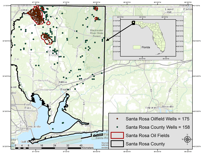
Figure 1. Study area in West Florida.
2.2. Disturbance Metrics and Building the Model
Calculating disturbance metrics began after infrastructure accounting was completed. This task was only possible by referring to historical and current remotely sensed images (air photos and satellite imagery) of the study area to visually confirm all roads had been accounted and separated into oil and non-oil. Imagery was also needed to find and digitize the central production facilities and well pads, which did not exist in our datasets.
A next task was to assign widths to oil and non-oil roads found in the oil blocks. For non-oil roads, widths were determined using data from [44] and [45] road datasets. Non-oil road widths fell into three categories: major roads, other major roads, and secondary roads. Their width ranged 7.32 - 24.00 m and these values were used to calculate the direct effects created on the landscape by the presence of infrastructure features; the amount of land directly taken up by the existence of infrastructure. Meanwhile, indirect (edge) effect zones were based on the European Environment Agency’s report on landscape fragmentation in Europe [50] , a thorough study of how roads fragment landscapes, and relevant policy implications. Indirect effects encompass areas where ecological consequences extend outward from infrastructure features [33] [51] - [53] . Also known as road effect zones [35] [24] , this measure is used to determine disturbance that may not be “seen” but can affect landscapes and wildlife. Automobile pollution, invasive plant species entering the areas between roads and natural vegetation, the spooking of wildlife by noise, bird diversity, burn severity of forests, and microclimatic changes are examples of edge effects [54] - [59] . Here the effects spanned 17.32 - 44.00 m.
For oil features, metrics were defined by BLM studies of oil production in Florida (2008) and Wyoming (2010). BLM [6] divided disturbance measures into three categories: exploratory, construction and production. Since all wells in our study area were established by 1990, oil infrastructure was deemed to be in the production phase. Based on BLM [6] figures, oil roads were assigned a 26.99 m width to represent direct effects. This closely compares to the 25 m direct effects calculated by [16] to accommodate oil infrastructure, right-of-way and buried pipelines in eastern Ecuador. To account for indirect effects, the BLM exploratory phase of 54.35 m disturbance was calculated. This was slightly more than double the size of direct effects, a strategy also used by [13] for computing oil-related edge effects in Ecuador.
In addition to roads, oil infrastructure included wells (rather than well pads) and central production facilities (which we digitized). The direct effects for wells, based on [6] figures, were 3,723 m2, while indirect were 13,071 m2. The direct effects for the production facilities, which were only found in Jay and Blackjack Creek oilfields, were based on the original size of the digitized footprint. The indirect effects were calculated by buffering the facilities by the same width used for indirect effects on oil roads. All oil features were then combined (roads, wells and production facilities) and disturbance measures calculated using ESRI’s ArcGIS model builder. When compared to non-oil infrastructure, oil infrastructure overcompensated for land disturbance, thus assuring us we were properly taking into account the role of oil alterations on the landscape. Based previous oil geospatial disturbance landscapes and landscape ecology metric studies [6] [13] [21] [28] [35] [61] , the infrastructure disturbance measures below were calculated and sequenced using ESRI ArcMap’s Model Builder.
Infrastructure length in km―separated into oil and non-oil.
Infrastructure density―this metric is a common way of determining the amount of habitat fragmentation (km/km2). Calculated for oil and non-oil.
Well density―number of wells per oilfield.
Direct effects―total amount of land occupied by oil and non-oil infrastructure features.
Indirect effects―buffered area of direct effects to accommodate edge effects. As Hartley et al. [61] note, this type of “effect zones enhances the credibility and viability of environmental analyses and decisions reached… by more accurately disclosing the direct, indirect, and cumulative impacts of fragmentation across the landscape.”
Core areas―these are the patches of intact natural vegetation that remain after discounting edge effect zones. They are “sufficiently far from transportation corridors to be relatively unaffected by them” [61] . They are therefore also known as roadless areas.
Land-use land-cover―classified into 8 categories. Percentage of each class was calculated for:
o The entire county.
o The oil fields.
o Direct and indirect effects specifically linked to oil and non-oil infrastructure features.
2.3. Land-Use
Land-use and land-cover maps were derived from NASS for the state of Florida and from datasets provided by SRCCPZDD. The former focused on land-cover (vegetation and structures that cover the land surface), while the latter focused on land-use (the human utilization of the landscape). The NASS raster file was converted to a vector file and clipped to Santa Rosa, and the 36 classes (many of them agricultural crops) were reclassified into eight (using ArcMap 10.1). These were: agriculture, barren, forest, shrub lands/grasslands, urban, water, wetlands and no data (see Figure 2).

Figure 2. Land use in the study area’s 6 oilfields. Note that agriculture occupies about 1/3 of the land, while natural areas (forest, grasslands and wetlands) take up about 57%.
The 24 Santa Rosa existing land-use groups were classified into nine categories and checked against the NASS data. The number of reclassified land-use and land-cover categories did not match up exactly between the two because the NASS classification scheme contained an additional 12 classes, mainly focused on distinct agricultural crops. Meanwhile the Santa Rosa land-use data included categories such as industrial, rail and utilities that we reclassified as urban. Vacant land, which could be classified as urban, stretched across large areas that also appeared forested in the NASS data, so we kept it as a separate category. Additionally, one large land-use, military, was also included in Santa Rosa data, for which there was no equivalent in the NASS data, and much of this is forested too.
The percentage of land dedicated to each category was computed for each oilfield and compared to the entire county. Then, to specifically understand the contribution to disturbance created by infrastructure features, the direct and indirect oil and non-oil datasets were extracted from the land-use maps of each oilfield and percentage values calculated. Finally, the core areas, natural areas remaining once the combined indirect effects for both oil and non-oil were discounted from the landscape, were calculated. For this study we calculated the size of core areas, as an important sustainability measure. Other researchers, however, have focused on core patch size, pattern and density as specific habitat fragmentation measures [8] [62] - [65] .
3. Results
3.1. Disturbance Metrics
Table 2 shows the values for the selected disturbance metrics. Jay was the largest field, around 46 km2; Blackjack Creek was half its size at about 19 km2. The remaining fields were less than 2.5 km2. Due to its larger size, more numerous wells and vaster infrastructure features both for oil and non-oil, Jay had the largest amount of disturbed land in terms of km2, followed by Blackjack Creek. Jay led with almost 60 km of oil roads and 101 km
Table 2. Landscape ecology disturbance metrics for study are oilfields.
of non-oil roads. With 136 wells, Jay had more than four times as many as Blackjack Creek, which had 29 wells. Naturally the direct and indirect disturbance values were also greatest in terms of overall land affected inside Jay, followed by Blackjack Creek. The disturbance values for the remaining four oilfields were much smaller. In fact, Coldwater Creek had no disturbances related to oil and gas activity.
A different pattern emerged, however, when landscape alterations were normalized by unit area, the oilfield, to create density measures. This time McClellan, with only three wells and its smaller size, had the highest oil road density at 1.59. Mt. Carmel was next at 1.41. Jay, by contrast had an oil road density of 1.3, the third highest, followed by Blackjack Creek (1.02), Sweetwater Creek (0.93). Coldwater had none.
In the study area, the highest well density was found in Mt. Carmel, with 4.11, indicating a disturbance of four wells per km2. Jay by contrast, with 27 times more wells but larger area, had a well density of 2.95, or almost three wells per km2. All, oilfields, except Coldwater Creek―which had no wells, had a well density greater than 1.
For non-oil road density, Blackjack Creek had the highest values (2.79), followed by Coldwater Creek (2.71). Jay had the third highest density at 2.20. It was followed by Sweetwater Creek (2.14), Mt. Carmel (1.78) and McClellan (1.59).
Road density values measure from 0.1 in remote areas to 40.0 in urban developed locations [13] [51] . Another road density measure, at the country level, is to take the linear km of road features and divide them by 100 km2 of land, where values range from 1 - 3850 [66] . Here, smaller countries, like smaller oil blocks, tend to have the highest road density values. For example, Monaco, Macao and Malta are at the top of the list, while larger countries such as the United States and China rank 52 and 69, respectively (when sorted from high to low).
Therefore, when calculating disturbance by unit area, the smaller oilfields tended to show high values for oil related direct and indirect effects. However, for non-oil related infrastructure, Jay and Blackjack Creek showed the highest values due to these areas being more developed―as evidenced by more roads and proximity to the town of Jay, Florida.
Finally, when combining oil and non-oil disturbances, Jay showed the highest values, but was followed by the smaller fields of Mt. Carmel and McClellan. Combining overall disturbance measures, both for direct and indirect effects is useful for land managers when planning expansion of extractive activities (see Figure 3).
Finally, core areas represent the amount of natural vegetation that remains after all infrastructure features are combined, buffered and erased from the oilfield. Also known as roadless3 areas, this measure is a proxy for undisturbed land and can be used to “assess the degree of fragmentation” [35] . By this measure, the greater the size of core areas in an oilfield, the less disturbed it is.
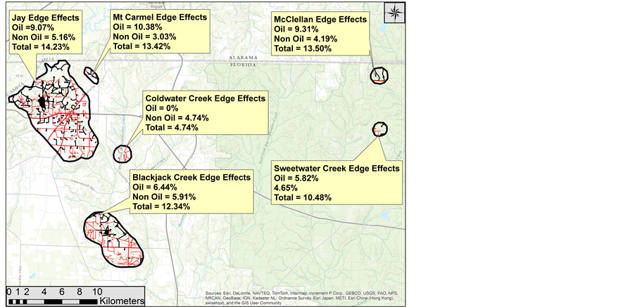
Figure 3. Indirect, or edge effects for oil and non-oil infrastructure in the study area’s six oilfields.
When calculating these areas, however, not only did we discount the indirect effects of infrastructure, we went a step further and excluded any remaining NASS land use that was not considered a natural area, such as urban and agricultural land. The categories that were left included: forest, shrublands/grasslands, water and wetlands. While these areas may not be connected (i.e. are missing wildlife corridors), they still provide sizeable portions of natural areas.
Two thirds of the oil fields had more than 60% of their land comprised of core areas. The lowest amounts were Mt. Carmel with 35% and Jay with 45%. For an oilfield as large as Jay, with the amount of built environment it contains, maintaining almost half of its land as core natural areas, is interesting. A further examination of the oil wells revealed that 22 of them had a status of dry hole and 10 were never drilled. Removing these wells from the calculated disturbance regime may have increased the size of core areas. However, we did not eliminate them earlier because some “defunct” oil wells were located on existing well pads, which were polygons of cleared land. The large amount of core areas does suggest that conservation of land was important to the land managers operating the oil fields and/or Santa Rosa County leaders (Figure 4(a) and Figure 4(b)).
3.2. LULC and Infrastructure
3.2.1. Land-Use Land-Cover
The dominant land-use in Santa Rosa County based on [67] data was silviculture-natural and managed forests, accounting for 31% of the county. Agriculture comprised about 12% of the county. Surprisingly, military occupied about the same amount of land as agriculture at 11.15%, though a lot of the land cover is forested. Urban followed at almost 9%; vacant at 7%; infrastructure was around 2%; and water less than 1%.
As a subset, the 6 oilfields combined showed that about 81% of land was dedicated to two uses: silviculture (47%) and agriculture (34%). Urban followed at 10%, while the other three classes, recreation/open land, vacant and infrastructure comprised less than 5% each. Silviculture and agriculture dominated in the largest two oilfields, Jay and Blackjack Creek, with greater amounts of silviculture. However, the two neighboring, but much smaller oilfields, Mt. Carmel and Coldwater Creek exhibited higher amounts of agriculture than silviculture, despite being less than 2 km away from Jay.
The key finding is that agricultural land predominates in the northwestern part of the county, where the large oilfields lie; helping confirm this area was an agricultural zone before oil was discovered [68] - [71] . The strong presence of silviculture, part of which is managed forests (pine plantations) also supports this finding. The dominant crops grown here are peanuts and cotton [72] .
Table 3 shows land-use land-cover values for the six oilfields and the entire county based on NASS data grouped into eight classes. Forest comprised about 54% of Santa Rosa County, followed by wetlands (13.63%) and urban and agriculture. These last two were practically tied around 11.50%.
In Blackjack Creek, forest (38.05%) and agriculture (25.41%) dominated, while wetlands still comprised
 (a)
(a)
 (b)
(b)
Figure 4.(a) and (b). The pattern and size of core areas for Jay, Mt. Carmel Coldwater Creek (a), and Blackjack Creek (b). The green areas are natural areas, forest and wetlands. The white areas include zones that have been disturbed by infrastructure, urbanization and agriculture.
Table 3. NASS land-use land-cover inside oil fields and county-wide.
about 20%. In Coldwater Creek, agriculture (30.01%), forest (28.07%) and wetlands (25.25%) were the most important categories. In Jay, agriculture occupied almost 41% of the area; the leading land use. This was followed by forest at almost 27% and wetlands at around 16%. This finding supports observations that the area around Jay was converted to agriculture before oil was discovered. In McClellan 90% was forest, while in Mt. Carmel 54% was agriculture and 25% forest. Sweetwater Creek was largely forested at 84%.
3.2.2. Land Use and Infrastructure
While calculating and mapping the amount of land directly and indirectly affected by infrastructure features is useful for understanding proportions and distribution of alterations per oilfield, it does not tell what type of land features have been affected. We therefore extracted these effects from the NASS land-use land-cover map to determine how oil and non-oil contributed to loss of natural areas or how they were intertwined with the built environment (see Figure 5).
Tables 4-8 show the type and amount of land cover occupied by the direct and indirect presence of oil and non-oil infrastructure features. In Blackjack Creek almost a third of oil-related structures were located in agri-

Figure 5. The land-use land-cover occupied by the indirect (edge) ef- fects of all infrastructure features (oil and non-oil combined) for Jay, Mt. Carmel and Coldwater Creek. Note that the yellow sections indi- cate infrastructure that is located in agricultural areas. The green shows infrastructure that runs through forested zones. The black only provides a background so that the indirect effects are visible.
Table 4. Land-use land-cover direct effects for oil infrastructure.
Table 5. Land-use land-cover direct effects for non-oil infrastructure.
Table 6. Land-use land-cover indirect effects for oil infrastructure.
Table 7. Land-use land-cover indirect effects for non-oil infrastructure.
Table 8. Core areas.
cultural zones. Shrublands were next, followed by urban and then forest, at about 16%. In Jay, about a third of oil features were also located in agricultural areas, while urban at 28%, was next. Thus approximately 2/3 of oil infrastructure was located in areas already disturbed. About 20% of these features ran through forests, showing the expansion of oil spreads beyond the built and agricultural environment. Mt. Carmel also had half of its oil features running through agriculture and 1/4 through forest. Meanwhile, the eastern McClellan and Sweetwater Creek’s oil infrastructure ran mainly through forest because these fields were mostly forested to begin with.
For non-oil infrastructure, forest, urban and agriculture were the predominant LULCs affected. Sweetwater Creek had the highest percentage of forest disturbed by non-oil infrastructure. Blackjack Creek, Coldwater Creek, McClellan and Mt. Carmel had 40% or more forest disturbed, while Jay, had about 17%. For the latter, about 40% of its non-oil infrastructure ran through urban land-use (see Table 5 and Table 7).
When considering edge effects (where infrastructure features were wider than the direct effects), the type of affected land remained mostly the same. Buffered features did not expand into new land use categories, suggesting a steady pattern for existing land uses, despite the presence of roads.
4. Conclusions/Discussion
The objective of this work was to understand the contribution of nonrenewable resource extraction in landscape alterations, particularly as oil and gas development and fracking expand in Florida and throughout the US [73] . We utilized an accounting from above approach that relied on remote sensing and GIS techniques to map and measure land surface disturbances related to oil and gas exploration and production activities (OGEPA) in six West Florida oilfields. This type of approach is well suited for determining alterations at the landscape level and can be done longitudinally if sufficient imagery is available, particularly at a high spatial resolution.
In fact baseline studies are recommended, whereby all surface alterations are accounted through remotely sensed data and GIS techniques prior to an extractive industry entering an area [7] [17] . This not only allows for better planning of exploration and production activities, but also helps land managers avoid sensitive areas and indigenous zones, helping reduce future legal liability
By calculating and examining the spatial distribution of both direct effects and indirect (edge) effects caused by infrastructure features and relating them to land-use and land-cover, we found that OGEPA had a small contribution to surface disturbance in West Florida. Agriculture has a longer history in Santa Rosa County and was the leading driver of LULC change. Additionally, forested areas were not necessarily natural forests, since silviculture is widely practiced in the study area. This means that alterations to forests may be classified as interruptions to agricultural areas rather than to natural landscapes.
By using disturbance measures drawn from landscape ecology, it is possible to quantify the contribution of each category, and to sum and rank these values in order to gauge sustainability of extractive activities in each location. These sustainability values can then be used to fortify environmental performance standards.
For example, when disturbance scores for the following categories were combined (well density, oil road density, non-oil road density, oil direct effects, non-oil direct effects, oil edge effects, non-oil edge effects, combined direct and indirect edge effects for oil and for non-oil), Jay scored the highest, meaning it had the most disturbance. It was followed by Blackjack Creek, Mt. Carmel, McClellan, Sweetwater Creek and Coldwater Creek.
When land-use land-cover disturbances were summed and ranked, Blackjack Creek and Jay were no longer the most disturbed, they ranked third and fourth respectively. The least disturbed oilfield was Sweetwater Creek; the most Coldwater Creek. Finally, when all disturbances (landscape metrics and land-use land-cover) were combined, summed and ranked, the most sustainable was Coldwater Creek and the least Blackjack Creek (see Table 9).
Some implications of this study include: when OGEPA disturbance was quantified and mapped for Santa Rosa’s six oilfields, the infrastructure related to this extractive activity was relatively minor. The most amount of land affected was 10% (in Mt. Carmel). This means that 90% or more of each oilfield was not affected by OGEPA, when the wider indirect effects were calculated. On the other hand, agricultural activities and non-oil infrastructure also created surface alterations in the oilfields―since oil and gas are not the only economic activities or land-uses in this zone.
Non-oil infrastructure did create a smaller footprint than oil, though the road widths used for calculating disturbance values were narrower than for oil, which considered not only the roads, but wells, pipelines and production facilities. Nevertheless, most of the land in each oilfield remained unaffected by all infrastructure features combined at their widest extent. For example, Jay, the field most disturbed, still had 86% of its area untouched by infrastructure.
Therefore, if OGEPA activities continue in Florida and the amount of disturbance remains similar to past alterations, then future landscape disruption will remain small. The most recent permit application for oil drilling in Jay occurred in May 2014 [74] .
By contrast a state like Colorado, with 103,000 wells [75] and a well density of 0.23, has OGEPA in 57 of its 64 counties. In fact Weld County in the northern part of the state has a well density of 1.66 (see Figure 6). Furthermore, with the growth of fracking in this country, the time is now for applying accounting for above approaches to infrastructure footprint accounting as a way to better manage, monitor and understand environmental disturbance related to extractive activities.
Table 9. Overall disturbance metrics and land-use land-cover ranks.

Figure 6. Oil well density in Colorado, 2013. Note how Weld County in the northern part of the state has the highest well density, at 1.66.
Acknowledgements
The authors thank Mary Ann Vance from the Santa Rosa County Community Planning, Zoning and Develop- ment Division for land use data sets and historical background information for Santa Rosa County; Robert C. Jordan, Kirt Brayshaw, Verónica Pérez and Germán Pérez from the University of North Florida for help with data acquisition and initial analysis. We also thank Daniel Johns, GIS Manager at Clay County Utility Authority in Florida for help with GIS analysis, and James M. Ellis, from Ellis Geospatial for help with remote sensing and GIS techniques. We are also grateful to the Environmental Center at the University of North Florida for providing a Seed Grant to help fund research and student work that contributed to this paper. Thank you to the anonymous reviewers who offered useful comments to this paper.
References
- Spenser, A. (2013) New Frontier: A Once-Booming Florida Oil Industry Tries to Get Back to the Past. The Barrel. Platts. http://blogs.platts.com/2013/01/07/florida_oil/
- FDEP (Florida Department of Environmental Protection) (2010) Permitted Oil and Gas Wells. http://www.dep.state.fl.us/gis/datadir.htm
- FDEP (Florida Department of Environmental Protection) (2014) Mining, Mitigation and Delineation―Oil and Gas Current Applications. http://www.dep.state.fl.us/water/mines/oil_gas/drill-apps.htm
- Temple, B. (2012) Sunniland Shale―An Emerging South Florida Basin Liquids Play. Oil and Gas Journal. http://www.ogj.com/articles/print/vol-110/issue-3/exploration-development/sunniland-shale-an-emerging.html
- FDEP (Florida Department of Environmental Protection) (2010) Oil and Gas Annual Production Reports. http://www.dep.state.fl.us/water/mines/oil_gas/production.htm
- BLM (Bureau of Land Management) (2008) Florida: Reasonably Foreseeable Development Scenario for Fluid Minerals. http://www.blm.gov/pgdata/etc/medialib/blm/es/jackson_field_office/planning/planning_pdf_florida.Par.65103.File.pdf
- Ellis, J.M. (2013) Personal Communication. Ellis-Geospatial. http://www.ellis-geospatial.com
- Reddy, C.S., Sreelekshmi, S., Jha, C.S. and Dadhwal, V.K. (2013) National Assessment of Forest Fragmentation in India: Landscape Indices as Measures of the Effects of Fragmentation and Forest Cover Change. Ecological Engineering, 60, 453-464. http://dx.doi.org/10.1016/j.ecoleng.2013.09.064
- Musakwa, W. and Van Niekerk, A. (2013) Implications of Land Use Change for the Sustainability of Urban Areas: A Case Study of Stellenbosch, South Africa. Cities, 32, 143-156. http://dx.doi.org/10.1016/j.cities.2013.01.004
- Clover, J. and Eriksen, S. (2009) The Effects of Land Tenure Change on Sustainability: Human Security and Environmental Change in Southern African Savannas. Environmental Science and Policy, 12, 53-70. http://dx.doi.org/10.1016/j.envsci.2008.10.012
- Turner II, B.L. (2010) Sustainability and Forest Transitions in the Southern Yucatán: The Land Architecture Approach. Land Use Policy, 27, 170-179. http://dx.doi.org/10.1016/j.landusepol.2009.03.006
- Musinsky, J.N., Reining, C.C.S., Rosenfeld, A.B. and Thomsen, J.B. (1998) An Analysis of Human Settlement along the Xan Oil Road in Laguna del Tigre National Park, Guatemala. Society of Petroleum Engineers.
- Baynard, C.W., Ellis, J.M. and Davis, H. (2012) Evaluating Disturbance of E&P Access Roads. ESRI News for Petroleum, 2012, 6-7. http://www.esri.com/library/newsletters/petroleum-perspectives/petrol-spring-2012.pdf
- Baynard, C.W., Ellis, J.M. and Davis, H. (2013) Roads, Petroleum and Accessibility: The Case of Eastern Ecuador. GeoJournal, 78, 675-695. http://dx.doi.org/10.1007/s10708-012-9459-5
- Wassertrom, R. and Southgate, D. (2013) Deforestation, Agrarian Reform and Oil Development in Ecuador, 1964- 1994. Natural Resources, 4, 31-44. http://dx.doi.org/10.4236/nr.2013.41004
- Hutton, W.C. and Skaggs Jr., M.M. (1995) Renewable Resource Development in the Ecuadorian Rainforest. Society of Petroleum Engineers 30684, 441-454.
- Janks, J.S., Prelat, A.E. and Wieser, J.D. (1994) Remote Sensing Technology Applications to Environmental Assessments in the Oriente Region of Ecuador. The 2nd Thematic Conference on Remote Sensing for Marine and Coastal En- vironments, New Orleans, 31 January 1994.
- Hiraoka, M. and Yamamoto, S. (1980) Agricultural Development in the Upper Amazon of Ecuador. Geographical Review, 70, 423-455. http://dx.doi.org/10.2307/214077
- Metzger, J.P. (2001) Effects of Deforestation Pattern and Private Nature Reserves on the Forest Conservation in Settle- ments Areas of the Brazilian Amazon. Biota Neotropica, 1, 1-14.
- Southworth, J., Marsik, M., Qiu, Y., Perz, S., Cumming, G., Stevens, F., Rocha, K., Duchelle, A. and Barnes G. (2011) Roads as Drivers of Change: Trajectories across the Tri-National Frontier in MAP, the Southwestern Amazon. Remote Sensing, 3, 1047-1066. http://dx.doi.org/10.3390/rs3051047
- Baynard, C.W. (2011) The Landscape Infrastructure Footprint of Oil Development: Venezuela’s Heavy Oil Belt. Ecological Indicators, 11, 789-810. http://dx.doi.org/10.1016/j.ecolind.2010.10.005
- Mjachina, K.V., Baynard, C.W. and Chibilyev, A.A. (2013) Oil and Gas Development in the Orenburg Region of the Volga-Ural Steppe Zone: Qualifying and Quantifying Disturbance Regimes. International Journal of Sustainable Development and World Ecology, 21, 111-126. http://dx.doi.org/10.1080/13504509.2013.867908
- Thomson, J.L., Schaub, T.S., Culver, N.W. and Aengst, P.C. (2005) Wildlife at a Crossroads: Energy Development in Western Wyoming. Effects of Roads on Habitat in the Upper Green River Valley. The Wilderness Society, Washington DC, 40 p. http://wilderness.org/sites/default/files/wildlife-at-crossroads-report.pdf
- Weller, C., Thomson, J., Morton, P. and Aplet, G. (2002) Fragmenting Our Lands: The Ecological Footprint from Oil and Gas Development―A Spatial Analysis of a Wyoming Gas Field. The Wilderness Society, Washington DC, 1-24. http://www.sagebrushsea.org/pdf/TWS_Fragmenting_Our_Lands.pdf
- Jankowitz, R. (2007) Oil and Gas Development Guidelines: Conserving New Mexico’s Wildlife Habitats and Wildlife. New Mexico Department of Game and Fish, 38 p. http://www.wildlife.state.nm.us/documents/oilandgasguidelines.pdf
- Morton, P., Weller, C. and Thomson, J. (2002) Energy & Western Wild Lands: A GIS Analysis of Economically Reco- verable Oil and Gas. The Wilderness Society, Washington DC, 31 p. http://grist.files.wordpress.com/2011/08/energy-wildlands-economic-analysis.pdf
- Morton, P., Weller, C., Thomson, J., Haefele, M. and Culver, N. (2004) Drilling in the Rocky Mountains: How Much and at What Cost. The Wilderness Society, Washington DC, 33 p. http://wilderness.org/sites/default/files/Drilling-in-the-Rocky-Mountains.pdf
- Wilbert, M., Thomson, J. and Culver, N.W. (2008) Analysis of Habitat Fragmentation from Oil and Gas Development and Its Impact on Wildlife: A Framework for Public Land Management Planning. The Wilderness Society, Washington DC, 31 p. http://www.fws.gov/southwest/ES/Documents/Oil-Gas-Fragmentation-Wilbert%20et%20al%202008.pdf
- McEnroe, M. and Sapa, A. (2011) Observations and Recommendations to Reduce Fish and Wildlife Impacts from Oil and Gas Development: A Report to the Membership of the North Dakota Chapter of the Wildlife Society. Bismark, 20 p. http://joomla.wildlife.org/NorthDakota/images/Documents/oilgas11.pdf
- Schneider, R. and Dyer, S. (2006) Death by a Thousand Cuts: Impacts of in Situ Oil Sands Development on Alberta’s Boreal Forest. Canadian Parks and Wilderness Society and the Pembina Institute, Edmonton, 36 p.
- Holroyd, P., Dyer, S. and Woynillowicz, D. (2007) Haste Makes Waste: The Need for a New Oil Sands Tenure Regime: Oil Sands Issue Paper No. 4. The Pembina Foundation, Drayton Valley, 35 p. http://www.pembina.org/pub/1409
- Florida Trend (2012) Florida’s Economic Makeup 2010. http://www.floridatrend.com/article/223/floridas-economic-makeup
- Watson, M.L. (2005) Habitat Fragmentation and the Effects of Roads on Wildlife and Habitats. New Mexico Department of Game and Fish, 1-18. http://www.wildlife.state.nm.us/conservation/habitat_handbook/documents/2004EffectsofRoadsonWildlifeandHabitats.pdf
- Wildlife Society (2012) Impacts of Crude Oil and Natural Gas Development on Wildlife and Wildlife Habitat in the Rocky Mountain Region: Technical Review 12-02. In: Bookhout, T.A., Ed., Bethesda, 45 p. http://wildlife.org/documents/technical-reviews/docs/Oil%20and%20Gas%20Technical%20Review_2012.pdf
- Wilderness Society (2006) Habitat Fragmentation from Roads: Travel Planning Methods to Safeguard Bureau of Land Management Lands. The Wilderness Society, Washington DC, 16 p. https://partners.tws.org/wildscience/Publications1/Habitat%20Fragmentation%20from%20Roads.pdf
- Baynard, C.W. (2013) Remote Sensing Applications: Beyond Land-Use and Land-Cover Change. Advances in Remote Sensing, 2, 228-241. http://dx.doi.org/10.4236/ars.2013.23025
- Liroff, R.A. (2012) A Roadmap for Addressing Environmental and Social Issues Associated with Horizontal Drilling and Hydraulic Fracturing. Journal of Petroleum Technology, 60-63. http://www.spe.org/industry/docs/RDChallengeLiroffEnvironment.pdf
- Liroff, R.A. (2011) Extracting the Facts: An Investor Guide to Disclosing Risks from Hydraulic Fracturing Operations. ICCR, New York, IEHN, Falls Church, 33 p. http://disclosingthefacts.org/Extracting-the-facts.pdf
- Gold, R. (2014) The Smart Way to Do Frackling. The Wall Street Journal, Saturday/Sunday, April 5-6, C3.
- ESRI (Environmental Systems Resources Institute) (2014) ArcGIS for Desktop Software. Redlands.
- Mathieu, P.P. (2010) Sustainable Development Using Earth Observations. Imaging Notes, 25. http://www.imagingnotes.com/go/article_freeJ.php?mp_id=241
- LABINS (Land Boundary Information System) (2013) Mapping Data. http://data.labins.org/2003/
- Lloyd, J.M. and Tootle, C.H. (1991) Information Circular No. 107. Part I: 1988 and 1989 Florida Petroleum Production and Exploration. Florida Geological Survey.
- FGDL (Florida Geographic Data Library) (2013) http://www.fgdl.org/metadataexplorer/explorer.jsp
- FDOT (Florida Department of Transportation) (2014) TranStat/GIS. http://www.dot.state.fl.us/planning/statistics/gis/
- USDOT FHA (United States Department of Transportation) Federal Highway Administration (2007) Mitigation Strategies for Design Exceptions. Chapter 3, the 13 Controlling Criteria. http://safety.fhwa.dot.gov/geometric/pubs/mitigationstrategies/chapter3/3_lanewidth.htm
- University of Florida Map Library (2013) Aerial Photography: Florida. http://ufdc.ufl.edu/aerials
- Babcock, C. (1991) Information Circular No. 107. Part II: Petroleum Exploration and Development Policies in Florida: Response to Public Concern for Sensitive Environments. Florida Geological Survey. http://ufdcimages.uflib.ufl.edu/UF/00/00/11/68/00001/UF00001168.pdf
- FGS (Florida Geological Survey) (2007) Organizational Highlights and Significant Historical Events of the Florida Ge- ological Survey. http://www.google.com/url?sa=t&rct=j&q=&esrc=s&source=web&cd=2&ved=0CCoQFjAB&url=http%3A%2F%2Fwww.dep.state.fl.us%2Fgeology%2FCentennial%2FHIGHLIGHTS%2520AND%2520SIGNIFICANT%2520EVENTS.doc&ei=E-SVU-DqOPTLsQSwhILAAQ&usg=AFQjCNHd-Ba3gZsowlIjDtEXG4SW_89umg&bvm=bv.68445247,d.cWc
- EEA (European Environment Agency) (2011) Landscape Fragmentation in Europe: Joint EEA-FOEN Report. Copenhagen. http://www.eea.europa.eu/publications/landscape-fragmentation-in-europe
- Forman, R.T.T., Sperling, D., Bissonnette, J.A., Clevenger, A.P., Cutshall, C.D., Dale, V.H., Fahrig, L., France, R., Goldman, C.R., Heanue, K., Jones, J.A., Swanson, F.J., Turrentine, T. and Winter, T.C. (2003) Road Ecology: Science and Solutions. Island Press, Washington DC.
- Culver, N. and Slivka, J. (2012) Designating Wildlife Corridors on the Public Lands―Protection through BLM’s Land Use Planning Process. The Wilderness Society, Washington DC, 1-24. http://wilderness.org/sites/default/files/Wildlife%20Corridors%20Brief%20-%20Feb%202012.pdf
- Coffin, A.W. (2007) From Roadkill to Road Ecology: A Review of the Ecological Effects of Roads. Journal of Transport Geography, 15, 396-406. http://dx.doi.org/10.1016/j.jtrangeo.2006.11.006
- Nayaranaraj, G. and Wimberly, M.C. (2013) Influences of Forest Roads and Their Edge Effects on the Spatial Pattern of Burn Severity. International Journal of Applied Earth Observation and Geoinformation, 23, 62-70. http://dx.doi.org/10.1016/j.jag.2012.12.006
- Delgado, J.D., Arroyo, N.L., Arévalo, J.R. and Fernández-Palacios, J.M. (2007) Edge Effects of Roads on Temperature, Light, Canopy Cover, and Canopy Height in Laurel and Pine Forests (Tenerife, Canary Islands). Landscape and Urban Planning, 81, 328-340. http://dx.doi.org/10.1016/j.landurbplan.2007.01.005
- Marcantonio, M., Rocchini, D., Geri, F., Bacarao, G. and Amici, V. (2013) Biodiversity, Roads and Landscape Fragmentation: Two Mediterranean Cases. Applied Geography, 42, 63-72.
- Batáry, P., Fronczek, S., Normann, C., Scherber, C. and Tscharntke, T. (2014) How Do Edge Effect and Tree Species Diversity Change Bird Diversity and Avian Nest Survival in Germany’s Largest Deciduous Forest? Forest Ecology and Management, 319, 44-50. http://dx.doi.org/10.1016/j.foreco.2014.02.004
- Gieselman, T.M., Hodges, K.E. and Vellend, M. (2013) Human-Induced Edges Alter Grassland Community Composition. Biological Conservation, 158, 384-392. http://dx.doi.org/10.1016/j.biocon.2012.08.019
- Avon, C., Bergès, L., Dumas, Y. and Dupouey, J.L. (2010) Does the Effect of Forest Roads Extend a Few Meters or More into the Adjacent Forest? A Study on Understory Plant Diversity in Managed Oak Stands. Forest Ecology and Management, 259, 1546-1555. http://dx.doi.org/10.1016/j.foreco.2010.01.031
- BLM (US Bureau of Land Management) (2010) Reasonable Foreseeable Development Scenarios for Oil and Gas Development in the Pinedale Field Office. http://www.blm.gov/pgdata/etc/medialib/blm/wy/programs/planning/rmps/pinedale/rfd.Par.68069.File.dat/02_Report.pdf
- Hartley, D.A., Thomson, J.L., Morton, P. and Schlenker-Goodrich, E. (2003) Ecological Effects of a Transportation Network on Wildlife: A Spatial Analysis of the Upper Missouri River Breaks National Monument. The Wilderness So- ciety, Washington DC, 1-27. http://wilderness.org/sites/default/files/Missouri-Breaks-Transportation-Effects-Full-Report.pdf
- Ogogo, A.U., Bisong, F.E. and Tawo, A.N. (2013) Habitat Fragmentation and the Population Status of Rodents in Abayum Forest, Ikom, Cross River State, Nigeria. Natural Science, 5, 914-918. http://dx.doi.org/10.4236/ns.2013.58110
- Vergara, P.M. and Hahn, I. (2009) Linking Edge Effects and Patch Size Effects: Importance of Matrix Nest Predators. Ecological Modeling, 220, 1189-1196. http://dx.doi.org.dax.lib.unf.edu/10.1016/j.ecolmodel.2009.02.015
- Teixido, A.L., Quintanilla, L.G., Carreño, F. and Gutiérrez, D. (2010) Impacts of Changes in Land Use and Fragmentation Patterns on Atlantic Coastal Forests in Northern Spain. Journal of Environmental Management, 91, 879-886. http://dx.doi.org/10.1016/j.jenvman.2009.11.004
- Aubad, J., Aragón, P. and Rodríguez, M.Á. (2010) Human Access and Landscape Structure Effects on Andean Forest Bird Richness. Acta Oecologica, 36, 396-402. http://dx.doi.org/10.1016/j.actao.2010.03.009
- World Bank (2014) Road Density (km of Road per 100 Sq. km of Land Area). http://data.worldbank.org/indicator/IS.ROD.DNST.K2/countries?display=map
- SRCCPZDD (Santa Rosa County Community, Planning, Zoning and Development Division) (2013) Existing Land Use Map (ELUM).
- Nelson, L.F. (2003) Reflections and a Salute to a Town Called Jay. Florida Historical Society. http://www.jayhistoricalsociety.org/pioneerstories/Reflections_and_a_Salute_to_a_Town_Called_Jay.pdf
- Jay Historical Society (2002) The Town of Jay Celebrates 100 Years―2002, Part 1. http://www.jayhistoricalsociety.org/pioneerstories/The_Town_of_Jay_Celebrates_100_Years_2002_Part1.pdf
- Jay Historical Society (2002) The Town of Jay Celebrates 100 Years―2002, Part 2. http://www.jayhistoricalsociety.org/pioneerstories/The_Town_of_Jay_Celebrates_100_Years_2002_Part2.pdf
- Diamond, J.T. (1949) Early Pioneers of Pine Level. Jay Historical Society. http://www.jayhistoricalsociety.org/pioneerstories/Early_Pioneers_of_Pine_Level_by_John_T_Diamond.pdf
- NASS (National Agricultural Statistics Service) (2013) Cropland Data Layer (CDL): Santa Rosa, Florida. http://nassgeodata.gmu.edu/CropScape/
- Allen, G. (2014) Oil Industry Gets an Earful as It Eyes Florida’s Everglades. National Public Radio (NPR). http://www.npr.org/2014/03/13/289423090/oil-industry-gets-an-earful-as-it-eyes-floridas-everglades
- FDEP (Florida Department of Environmental Protection) (2014) Mining, Mitigation and Delineation―Oil and Gas Current Applications. http://www.dep.state.fl.us/water/mines/oil_gas/drill-apps.htm
- COGCC (Colorado Oil and Gas Conservation Commission) (2014) GIS Online. http://cogcc.state.co.us/Downloads/WELL_SHP.ZIP
NOTES

1Jay is also the name of the town located nearby.
2An exception is the year 2009, when production drastically fell to about 225 b/d [5] .

3Legislatively, roadless also means “the absence of roads which have been improved and maintained by mechanical means to insure relatively regular and continuous use” [61] .