E-Health Telecommunication Systems and Networks
Vol.2 No.2(2013), Article ID:33798,12 pages DOI:10.4236/etsn.2013.22006
Dynamic Optimization of Caregiver Schedules Based on Vital Sign Streams
1NYC Social Network Research Group, John Jay College (CUNY), New York, USA
2Department of Math and Computer Science, John Jay College (CUNY), New York, USA
Email: msaad@snrg-nyc.org, bkhan@jjay.cuny.edu
Copyright © 2013 Mohamed Saad, Bilal Khan. This is an open access article distributed under the Creative Commons Attribution License, which permits unrestricted use, distribution, and reproduction in any medium, provided the original work is properly cited.
Received December 25, 2012; revised February 1, 2013; accepted May 1, 2013
Keywords: Critical Care; Nurse Scheduling; Optimization
ABSTRACT
Hospital facilities use a collection of heterogeneous devices, produced by many different vendors, to monitor the state of patient vital signs. The limited interoperability of current devices makes it difficult to synthesize multivariate monitoring data into a unified array of real-time information regarding the patients state. Without an infrastructure for the integrated evaluation, display, and storage of vital sign data, one cannot adequately ensure that the assignment of caregivers to patients reflects the relative urgency of patient needs. This is an especially serious issue in critical care units (CCUs). We present a formal mathematical model of an operational critical care unit, together with metrics for evaluating the systematic impact of caregiver scheduling decisions on patient care. The model is rich enough to capture the essential features of device and patient diversity, and so enables us to test the hypothesis that integration of vital sign data could realistically yield a significant positive impact on the efficacy of critical care delivery outcome. To test the hypothesis, we employ the model within a computer simulation. The simulation enables us to compare the current scheduling processes in widespread use within CCUs, against a new scheduling algorithm that makes use of an integrated array of patient information collected by an (anticipated) vital sign data integration infrastructure. The simulation study provides clear evidence that such an infrastructure reduces risk to patients and lowers operational costs, and in so doing reveals the inherent costs of medical device non-interoperability.
1. Introduction
Preventable, in-hospital medical errors account for between 100,000 and 200,000 deaths in the United States each year [1]. There have been many attempts to determine the underlying causes, including the reports of Health Grades, a leading healthcare ratings organization [2], and the Joint Commission, a non-profit organization seeking to improve safety through healthcare accreditations. A recent Joint Commission report, for example, investigates incidents of deaths and serious injuries related to long-term ventilation [3]. Of the incidents reviewed, approximately 20% - 35% were found to be associated with insufficient staffing levels and/or a delayed response to an alarm; none were related to ventilator malfunction.
The extent to which we can mitigate patient risks caused by delayed responses and insufficient staffing, rests on addressing the problem of effective caregiver scheduling. Notable prior work, including that of McManus et al. [4] and Zai et al. [5] has used queuing theory to model the operation of existing healthcare facilities and admission procedures. The existing practices of “manpower allocation” in respiratory care is considered by Matthews et al. in their 2006 study [6], while Gajc et al. examine the effects of having 24-hour (mandatory) versus on-demand critical care specialists on staff. All of these studies begin with data from existing facilities and analyze the data to build a model and determine how the model responds to various stresses. In contrast, other researchers (e.g. Gallivan et al. [7] and Shahani et al. [8]) look to improve workflow and decision making processes by mining data from existing CCUs. Indeed, the general problem of designing nurse scheduling algorithms has received considerable attention, including hierarchical [9], greedy [10], genetic, and simulate annealing approaches [11]. Here we connect the important problem of nurse scheduling to the practical implications of device heterogeneity and non-interoperability.
Hospitals use sophisticated equipment to monitor the state of patient vital signs such as body temperature, pulse rate, blood pressure, and respiratory rate [12]. In critical care, such equipment might additionally include ventilators for moving breathable air into and out of the patient’s lungs, infusion pumps for injecting fluids, medication and/or nutrients into a patient’s circulatory system, pulse oximeters for measuring the oxygen saturation levels in a patient’s blood stream, and cardio monitors for measuring the electrical and pressure waveforms of a patient’s cardiovascular system [13-15]. As summarized by Charles Friedman, it is a “Fundamental theorem of biomedical informatics” that “a person working in partnership with an information resource is better than that same person unassisted” [16]. In practice, however, a problem arises since patient vital sign data must be collected using a set of heterogeneous devices produced by a number of distinct manufacturers. Each of these devices has a corresponding, often proprietary, system of cabling and data protocols. As technology advances, the number of devices per patient grows, and it becomes increasingly more challenging for a caregiver to monitor information and alarms generated by each of the different devices, let alone integrate the multivariate information into a holistic picture of the patient’s overall health. Each vital sign monitor provides warning alarms, but device heterogeneity makes it difficult to prioritize alarms relative to each other [1]. The side effects of device diversity are amplified at the scale of the healthcare unit, where, as patient-to-nurse ratios increase, information monitoring becomes even more challenging, since caregivers must attend to ever greater numbers of patients.
Certainly there are ongoing efforts to standardize medical device interfaces, thereby allowing for easier integration in both critical care and operating rooms. Most of these approaches (e.g. COSMOS [17]) have sought to define data standards for interconnectivity between heterogeneous systems in healthcare [18]. A recent RFID based approach to device integration was demonstrated in pilot project in a Taiwan hospital [19]. Classical wireless solutions have also been explored (see, e.g. [20]). Such efforts aim to develop an infrastructure capable of integrating vital sign data streams, thereby providing a unified view of a collection of patients, synthesized from a diverse collection of medical devices. Proponents of such infrastructures claim they would yield great positive impacts on the delivery of critical care. Here we evaluate these claims quantitatively.
Outline. In this paper, we develop a formal mathematical model of a critical care facility. The model is rich enough to capture the essential features: An infinitely replenishable finite set of patients whose vital signs are monitored; a smaller set of caregivers capable of addressing alarm conditions. Patients who experience an alarm accumulate injury exponentially during the time that they are without a caregiver; the time it takes the caregiver to treat the underlying causes of the alarm is proportional to the accumulated injury prior to care. If a patient accumulates more than a threshold level of injury before a caregiver arrives to treat them, a fatality occurs. Fatalities (or “Code-Blue” events) require the execution of close out procedures, which take a specified period of time (and must be given precedence over handling alarms from current living patients). This model, suitably formalized, specifies six constraints (I-VI) which a valid scheduling system must satisfy. Using the formalisms of the model, we are able to express concrete performance metrics by which any caregiver scheduling algorithm may be evaluated. We then consider two caregiver scheduling algorithms which operate within the proposed model. The first represents the current defacto standard scheduling procedure carried out in most critical care facilities today. The second algorithm is one which could only be instrumented if a vital sign data integration infrastructure was available. The algorithms and performance metrics are instrumented as a computer simulation. Analysis of large numbers of simulations allows us to verify and quantify the expected benefits of a vital sign data integration infrastructure on critical care delivery.
2. System Model
The system model consists of three mechanisms: the patient, the caregiver, and the facility. Each of these is described separately in the subsections that follow.
2.1. Patient Model
A vital sign is a real-time measurement of a patient, modeled as a function v:  from time to a real vector space1. Many classes of vital signs arise in practice, because of biological and vendor diversity.
A patient p, then, is a collection of k(p) vital signs2, . The range space
  of each vital sign is typically partitioned into regions, based on the semantics of v. These disjoint regions are labeled with qualitative labels, such as: “normal”, “fatal”, etc. We can view the range
  of vital sign v, as the state space of a dynamical system, wherein vital sign v traces a trajectory (over time). The set of all points with the label “fatal” form a limit set within the dynamical system, and associated with this limit set is a basin of attraction. When the vital sign trajectory is determined to have entered the basin of attraction, an alarm is raised. An alarm is thus a triple (p, i, t) consisting of a patient p, a vital sign
 , and a time t ≥ 0. The occurrence of alarm (p, i, t) is an assertion that the state of vital sign i in patient p has attained a value, which if left unattended, is expected to lead to increasing patient injury (and ultimately death). We will often think of alarm a = (pa, ia, ta) as an incident concerning the state of vital sign ia of patient pa at time ta. The process of defining the limit sets (corresponding to fatal states) and their basins of attraction, is outside the scope of what we seek to model here. We assume basins of attraction are defined by medical practitioners, in coordination with manufacturers of health monitoring devices. The set of all alarms raised for vital sign i of patient p in the half-open time interval [t1, t2) is denoted A (p, i, t1, t2); we take A (p, i, t1, t2) = Æ when t2 ≤ t1.
Post-alarm, a patient accumulates injury as they move in a trajectory through the state space , towards the fatal limit set. In this work, we model the injury as exponential in elapsed time, as has also been adopted in prior research [21-23]. Thus, after alarm a = (pa, ia, ta) occurs, patient pa who remains unattended until time t accumulates injury given by:
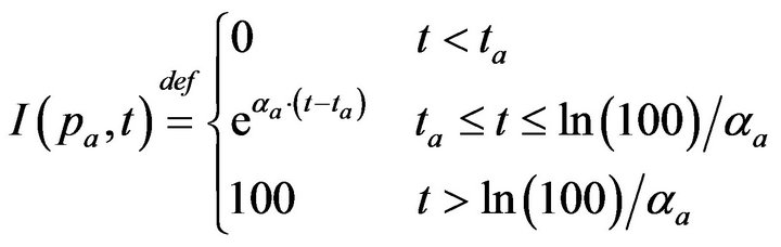
If the patient remains unattended for longer than Da = ln(100)/αa post-alarm a, injury reaches 100, signifying death. Each alarm a must therefore specify αa (or equivalently, its time until death Da). In our simulation experiments, we model all alarms involving vital sign i (regardless of patient), as sharing the same time until death, and so denote the common value as Di.
In this work, we model the alarms events for each vital sign at each patient as an independent Poisson process. More precisely, let (p, i, t1) and (p, i, t2) be two success-
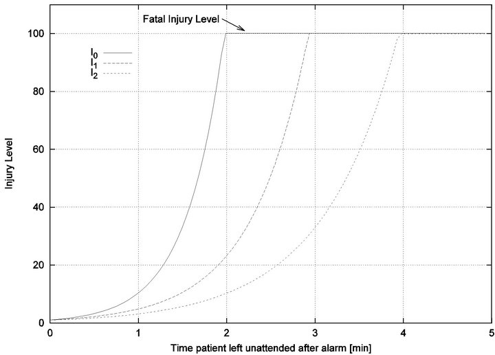
Figure 1. Injury functions for 3 different vital signs.
sive alarms, that is t1 < t2 and there is no alarm (p, i, t') for patient p’s vital sign i, where t1 < t' < t2: Then we assume that the alarm inter-arrival time t2 − t1 is a random variable that is distributed according to a Poisson distribution of intensity λp,i. In our experiments, we further assume that each of the patients exhibits the same alarm inter-arrival times for vital sign i, and thus, we will denote the common intensity as λi, and consider this number to be a characteristic property of the vital sign i itself, rather than the patient.
2.2. Caregiver Model
A caregiver is an individual capable of attending to the conditions underlying patient vital sign alarms. Associated with every patient p and caregiver c there is a caregiver assignment function h(p,c,t) {0,1}, where h(p,c,t) = 1 if and only if a caregiver c is attending to patient p at time t. The design of caregiver specific assignment functions h will be addressed in later sections. Here, we seek only to formally describe the constraints on h (and closely related functions), thereby specifying the requirements for valid assignment algorithms.
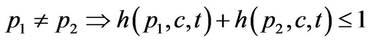
First, a caregiver c cannot be assigned to two distinct patients at the same time t; this is Condition I.
The set of times when patient p is being attended to by caregiver c, defined as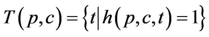 , is uniquely expressible as a disjoint union of maximal half open intervals; this is Condition II.

where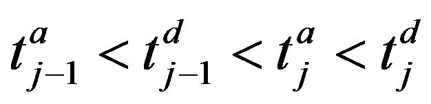 . The arrivals of caregiver c at patient p are a sequence
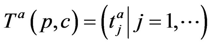 ; the departures are
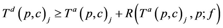
 . The jth arrival time of caregiver c at patient p is denoted Ta(p,c)j; the jth departure is denoted Td(p,c)j. We make a simplifying assumption, which at all times, at most one caregiver is assigned to patient p; this is Condition III.

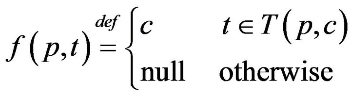
It follows that each patient p witnesses an interleaved sequence of caregiver arrivals and departures, allowing us to define the function f(p, t) as:
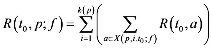
The times (prior to sometime t0) when patient p was served by (any) caregiver is denoted:
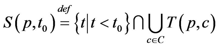
This permits us to define , which informally, is the last time (not later than t0) when patient p was serviced by any caregiver. At time t, each patient p has an associated (possibly empty) set of unresolved alarms
  We emphasize that the definition of X is dependent on the caregiver assignment function by listing f it as a parameter; we will follow this convention in later definitions as well.
2.2.1. Treatment Times
Having defined X, we can now turn to the process by which patient treatment occurs. If no caregiver is assigned to p at time t, then X(p,i,t;f) may be nonempty. Each alarm  contributes to the cumulative injury experienced by patient pa. Suppose that c is the first caregiver assigned to patient p at a time t0 > ta. We model the time required for c to address alarm a as being linearly proportional to the patient’s injury level. Formally
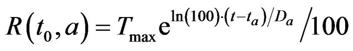
where Tmax is the maximum time required to resolve an alarm (as patient injury approaches 100). We model the treatment time as linearly additive for multiple alarms; the total time required for the caregiver c to handle all the alarms at patient p present at time t0 is then given by
For simplicity, we assume no preemption; that is, once a caregiver c has been assigned to patient p at time t0, the caregiver must remain with the patient for entire recovery period R(t0,p), regardless of other new (potentially more serious) alarms at other patients during that interval. Thus,
Once assigned, a caregiver stays with the patient until all alarms have been resolved, and the time required for treatment is linearly additive in injury level across all vital signs; this is Condition IV: for all time t between Ta(p,c)j and Ta(p,c)j + R(Ta(p,c)j, p; f ), g(c, t) = p.
2.3. Facility Model
The model described so far admits fatalities; these occur whenever caregivers fail to be present at patient pa in the interval between ta and ta + Da. In this section, we will formally describe the impact of fatalities on the scheduling of caregivers in a medical facility. When a fatality occurs, the expired patient is removed from the bed immediately, and placed in “Code-Blue” (CB) state which requires special close out procedures taking time Tfatal. To facilitate assignment of caregivers to the processing of Code-Blue cases, we introduce the caregiver-centric assignment function g, written as:
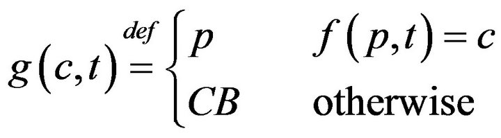
which associates each caregiver c and time t, with either a patient p Î P, or a special sentinel value CB indicating that caregiver is assigned to Code-Blue. We define s(c,j;g) to be the starting time of caregiver c’s jth assignment, defined by taking s(c,0;g) = 0, and then s(c, j+1;g) inductively, ta king it as
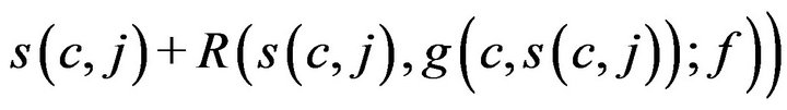
when g(c, s(c, j)) ≠ CB, and as s(c, j) + Tfatal otherwise.
If a caregiver is assigned to CB, they must complete the close out procedures (which require time Tfatal) before handling any new alarms. This is formalized in Condition V: If (j > 0) we have g(c, s(c, j)) = CB then for all t in between s(c, j) and s(c, j) + Tfatal, f (c; t) = CB.
When a fatality occurs, the model semantics are to transfer the expired patient to Code-Blue, and to populate the now-vacant bed with a new critical care patient. This new patient is the source of future alarms that are attributed to “patient p”.
2.3.1. Processing Fatalities
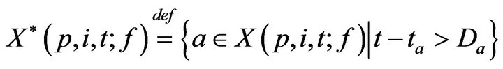
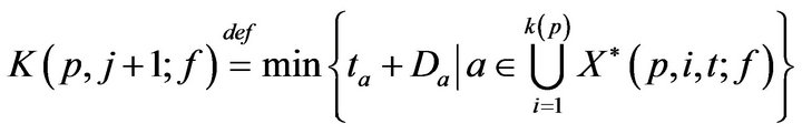
Towards accounting for fatalities, we define K(p, j; f) as the time of the jth fatality in bed p. K is defined inductively: As a base case, we take K(p, 0; f ) = 0. To express K(p, j+1; f ), recall that X(p, i, t; f ) is the set of unaddressed alarms which occurred for vital sign i (in bed p) at time t. Of these, we can describe the subset which induced a fatality.
Inductively then,
We define a monotonic integer valued function CB+(t;g) whose value is the size of the population admitted to the hospital Code-Blue. This can be expressed as
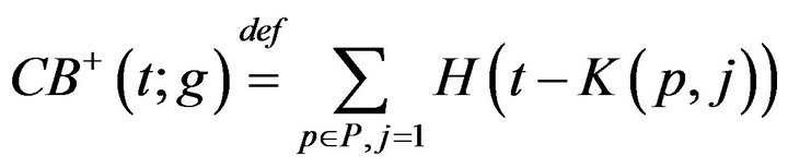
where H is the Heaviside step function. The number of times prior to t, when caregiver c was assigned to CB, denoted CB-(c,t;g), is given by
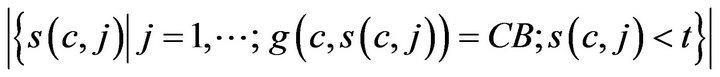
The number of times prior to t, when any caregiver was assigned to Code-Blue is
Thus, while CB+ (t) is the number of patients admitted to Code-Blue (prior to t), CB-(t) is the number caregivers assigned to Code-Blue (prior to t). Whenever the former quantity exceeds the latter, there is an unprocessed patient in Code-Blue. If caregiver, upon completing an assignment, determines that there is there is an unprocessed patient in Code-Blue (i.e. CB+ > CB-), they must be assigned to CB. This formalizes the fact that close out procedures for unprocessed fatalities must take precedence over the handling of existing critical care patients. Formally stated, this is Condition VI:
VIa If c is assigned to p at Ta(p,c)j (for some j), then c completes the assignment at .
. . Thus, if CB+ (ξ;g) > CB-(ξ;g) then it is required that g(c; ξ) =CB.
VIb If c is assigned to CB at time t0, then c completes the assignment at time ξ* = t0 + Tfatal. Thus, if CB+ (ξ*;g) > CB-(ξ*;g) then it is required that g(c; ξ*) = CB.
3. System Metrics
We now turn to the problem of evaluating a caregiver assignment algorithm. The jth assignment of caregiver c can either be (A) to a living patient, or (B) to the CB. Let us considered the incurred costs of each:
(A) If c is assigned to (living) patient p, then the cost C(c, j;g) incurred by the caregiver is linearly additive in injuries due to unhandled vital sign alarms at p, and represented by a multiset of real valued tokens
 (1)
(1)
where  is interpreted as a disjoint set union. While a caregiver is currently assigned to a patient p, alarms may continue to be generated at p. These alarms result in unit injury (via the exponential injury function, since e0 = 1), and hence unit tokens. Thus, the set (1) is augmented with a multiset of tokens each having value 1; these correspond to the costs of handling alarms which arose at p while c was at p. The augmented multiuset is denoted T (c, j).
(B) If c was assigned to the Code-Blue, then the cost C(c, j;g) incurred by the caregiver is taken as Cfatal, and T (c, j) is taken to be {Cfatal}.
Over the lifetime of the simulation, and the operation of the caregiver assignment algorithm A, each caregiver c collects a multiset of tokens , while the algorithm as a whole collects
 .
.
3.1. Cumulative Cost Metric
In general, we evaluate an algorithm A by analyzing properties of the tokens TA accumulated by the end simulations. One very crude measure of A’s performance is the total injury . In conducting multiple simulations, we will draw error bars around each curve to show the mean/variance of each algorithm’s performance over sets of trials. In comparing two algorithms A0 and A1, if we find that the mean curve of one algorithm lies within the error bars of another, then it is inconclusive which algorithm is superior (if any). What is needed in such settings it to understand the correlations (if any) between the two algorithms performance on specific input sequences. We assess this by considering the relative costs of the two algorithms over each of the trials.
3.2. Injury Histogram Metric
An algorithm which exhibits a large number of small injuries is not equivalent to one which exhibits a single fatality, though under the cost metric of the previous section, the two may be indistinguishable. Clearly, we need a fine grained scheme that allows us to keep track of the numbers of injury events (of various severity), rather than collapsing all injuries into a single uniform scalar value. To do this, we define a 5-band injury model, based on the injury curve:
• A Minimum Injury occurs if caregiver reaches patient before time  post-alarm a.
• A Medium Injury occurs if caregiver reaches patient between time  and
and  post-alarm a.
• A Critical Injury occurs if caregiver reaches patient between time  and
and  post-alarm a.
• A Major Injury occurs if caregiver reaches patient between time  and Da post-alarm a.
• A Fatal Injury occurs when caregiver reaches patient after time Da post-alarm a.
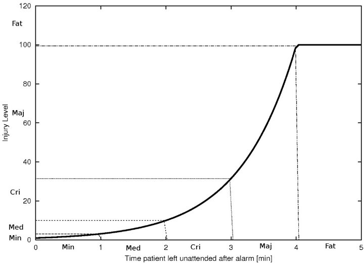
Figure 2. Identifying injury level bands.
4. Simulation Framework
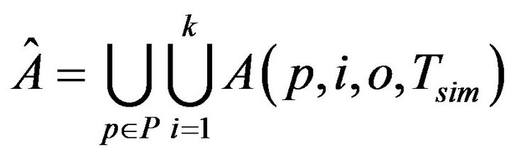
The first set of inputs to each assignment algorithm is a set of static configuration parameters. These include, the patients P, the caregivers C, the uniform time to death Di for each vital sign i=1,...,k; the maximum time to process an injury Tmax; the time (resp. cost) to process a fatality Tfatal (resp. Cfatal). The second set of inputs is dynamically generated, and consists of the entire sequence  of vital sign alarms that will be raised (for all vital signs, and all patients) in the course of the simulation. To generate Â, the simulator needs to be informed of the patients P, the number of patient vital signs k, the intensity of the Poisson process governing alarms for each vital sign λi, and the duration of the simulation Tsim. It then generates the alarms set A(p,i,0,Tsim) by sampling an independent Poisson processes of intensity λi. The cumulative set of alarms is:
The operation of the simulation software is depicted in Figure 3. Each algorithm A[i] will assign caregivers in response to the same sequence of alarms Â, according to its own criteria. During each algorithm’s execution, the caregivers collect a multiset of injury tokens, which are aggregated into a multiset T [i]. The statistical data analyzer, then analyzes all algorithm token multisets, and computes comparative metrics.
5. Proposed Algorithms
Caregiver scheduling is a real-time problem which shares some common ground with on-line algorithms, and the
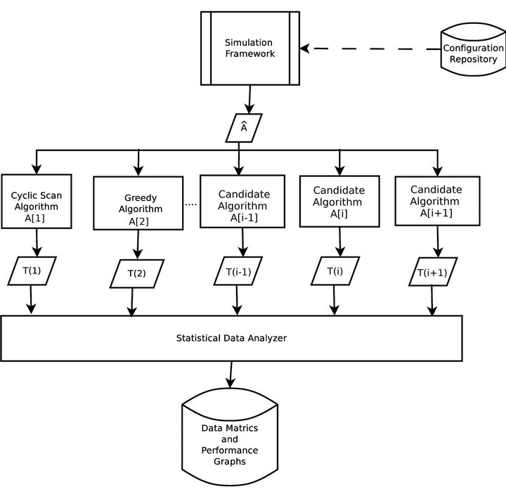
Figure 3. Simulation architecture.
generalizes paging and caching problems, and can be viewed as an on-line vehicle routing problem [24,25]. In contrast with the k-server problem, we do not require immediate handling of on-line requests (i.e. alarms). Our focus is not on competing against alarm sequences that have been crafted by a malicious adversary, but rather to analyze and quantify our system performance on an input sequences generated from specific probability distributions. In our comparative analyses we are designing algorithms which are able to leverage emerging vital sign integration infrastructures in order to outperform the defacto caregiver scheduling algorithms that are in use today.
5.1. Cyclic Scan (CS)
The Cyclic Scan algorithm (CS) represents a formalization of the defacto modus operandi of the majority of critical care units today. First, it reflects the absence of interoperability between vital sign monitoring devices: each device produces data in its own proprietary format, and data from heterogeneous devices cannot be integrated. Second, it reflects the absent of a wireless data communication infrastructure. These two features are the dominant norm in the healthcare industry today, and taken together, they reduce the task of monitoring patient vital signs to a process in which caregivers “can” among the patients’ monitoring devices to collect the presented data and status information. Figure 4 shows the flow chart for the CS algorithm.
5.2. Greedy
The Greedy algorithm is made possible by a vital sign integration infrastructure. Alarm data is consolidated wirelessly at a central location, and each caregiver is, as they become available, dispatched to the alarm which reports the highest injury level at that moment. It is designed to prioritize (triage) handling of alarms based on instantaneous patient injury levels.3
6. Experiment 1: One Caregiver
Objective. We seek to determine the maximum number of patients |P| that can be satisfactorily served by a single caregiver, and the dependency of this value on the alarm frequency λ and the maximum service time Tmax. We seek to quantify the impact of integrated vital sign data on the efficiency of a single caregiver.
Parameters. Thirty simulations were conducted for each system configuration. Each simulation was for 480 minutes (a standard work shift) in a facility with |C| = 1

Figure 4. The Cyclic Scan (CS) algorithm flow chart.
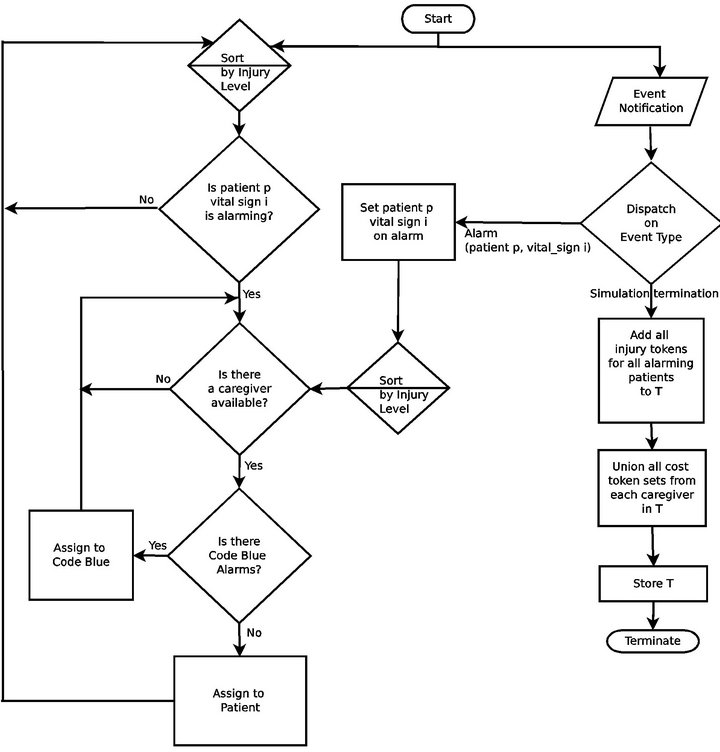
Figure 5. The Greedy algorithm flow chart.
caregiver. All patients had k =1 vital sign, whose alarms time to fatality was D1 = 6 minutes.
Experiment 1 has three parts. In Part 1, we varied |P|, the number of patients, while fixing the Poisson alarm process intensity λ1 = 20 minutes, and the maximum service time Tmax = 25 minutes and Code-Blue processing time Tfatal = 25 minutes. The results of Part 1 are considered the “baseline”. In Part 2 of the experiment, we varied the intensity λ1 = 7.5,15,40,80 minutes and studied the effects on performance against the baseline. In Part 3 of the experiment, we varied Tmax = Tfatal = 6.25, 12.5, 50, 100 minutes, and studied the effects on performance against the baseline.
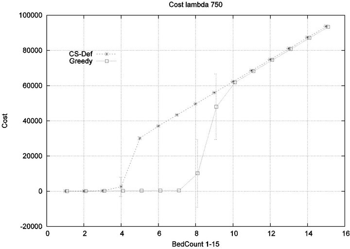
Part 1: Here, we seek to quantify how increasing the workload of a caregiver (i.e. the number of patient beds) impacts the emergence of injury within the critical care unit. Figure 6 shows that initially the cost of all algorithms is in agreement, since the workload of the caregiver is so low that optimization is unnecessary. This parity breaks down when the number of beds exceeds 4, as the Cyclic Scan sees a dramatic rise in cost from 0 to 17000 as the number of beds increases from 4 to 8. During this same interval, the Greedy algorithm maintains its lost cost. Finally, when the number of beds increases beyond 8, the Greedy algorithm begins to experience non-zero cost; at such high workloads, greedy scheduling cannot avoid the occurrence of patient injury. Finally, when the number of beds is sufficiently high, in excess of 13, the costs of the algorithms once again coincide, since greedy optimization is now no better than Cyclic Scan at circumventing patient injuries.
The reader may note that the Cyclic Scan algorithm experiences the start of a “phase transition” at 4 beds, while the Greedy algorithm begins the same phase transition at 9 beds. The algorithms complete their phase transition at 13 beds, at which point they re-merge with the performance curve of the naive Cyclic Scan.
The error bars (across multiple trials) tend to be small outside of the phase transition, but grow during phase transitions. This may lead the reader to question whether, the Greedy algorithm really outperforms the Cyclic Scan (for example in the 11 bed scenario), since the curves lie within a standard deviation of each other. The graph of Figure 7 seeks to address this concern. It depicts the relative performance of Greedy normalized against the Cyclic Scan. Note that the normalized performance is computed for each trial, and the graph depicts the mean and standard deviation of these normalized values.

Figure 6. Baseline absolute costs, Greedy vs. CS.
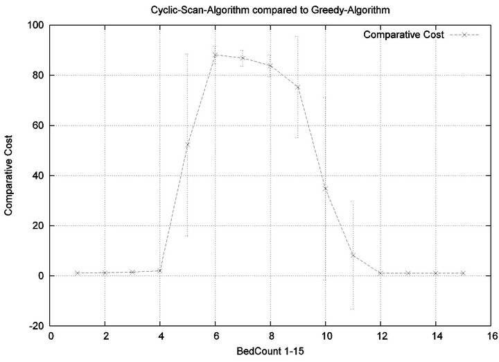
Figure 7. Baseline relative costs, Greedy vs. CS.
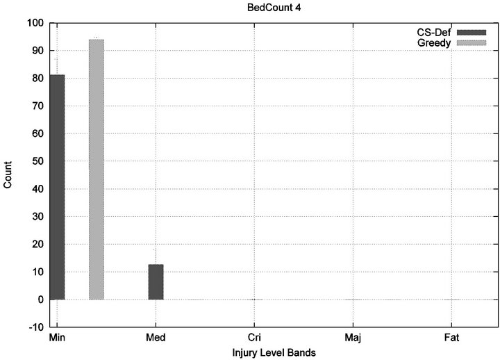
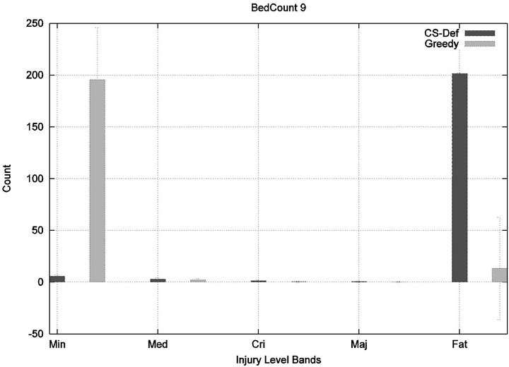
We see that each algorithm experiences a phase transition a critical number of beds at which the cost begins to rise. The question remains as to the nature of the underlying injuries? Are there many minor injuries, or a single Code-Blue, for example? The histograms in Figure 8 show that the phase transition for Cyclic Scan is rapid and bipolar. As the number of beds increases from 4 to 6, most of the costs incurred shift from minimal level injuries to Code-Blue injuries. At 4 beds, the injuries manifest at minimum and medium levels. At 5 beds (histogram not shown) there are injuries occurring at all levels. By 6 beds, the vast majority of injuries are at Code-Blue. The histograms in Figure 9 show that the Greedy algorithm, like Cyclic Scan, has a phase transition which also is rapid and bipolar. At 9 beds, the injuries manifest at minimum and medium levels. At 10 beds (histogram not shown), there are injuries occurring at all levels. By 11 beds, the vast majority of injuries are at Code-Blue.
It is clear from the prior fine-grained analysis, that both Greedy and Cyclic Scan keep cost low by uniformly keeping all injury levels low, but at some load threshold (i.e. when |P| becomes too large), both fail to be able to continue to achieve this, and are forced to trade off minimal level injuries for higher level injuries. The trade off phenomenon is made apparent in graph of Figure 10.
Part 2: Now we seek to quantify the influence of alarm frequency on the emergence of injuries within the critical care unit. In effect, we seek to quantify the impact of varying λ1 on the conclusions of Part 1.
We consider alarm sequences in which the mean interarrival time is varied between 7.5 min, 15 min, 40 min and 80 min; graphs for extreme values 7.5 min and 80 min are provided in Figure 11. We see that the Greedy algorithm incurs injuries when the bed count exceeds 7, 8, 9, and 10, for each of the scenarios. By comparison, Cyclic Scan incurs injuries whenever the bed count exceeds 4 - 5. Thus, the Greedy algorithm is able to leverage alarm sparsity towards a capacity to handle more patients
 (a)
(a) (b)
(b)
Figure 8. Cyclic-Scan’s injury phase transition.
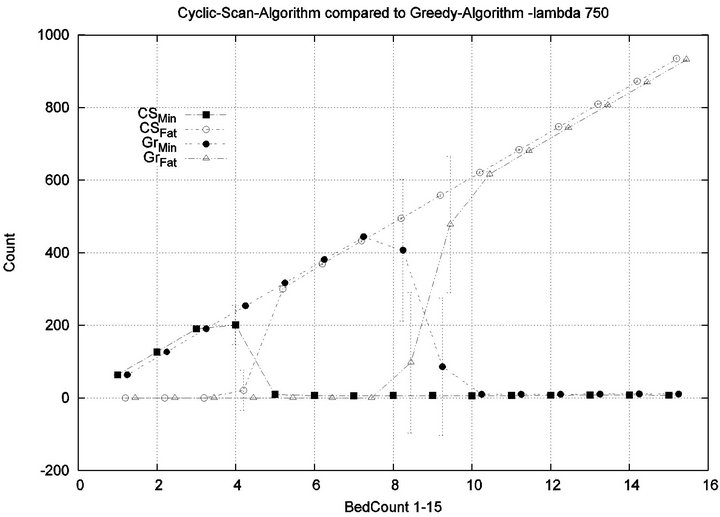
in an injury-free manner. The conclusion is further supported by considering the upper boundaries of the phase transition where the performance of two algorithms once again coincides. This occurs at bed counts 10, 11, 15, and 19 for the four respective scenarios. Thus, the size of the interval (in terms of bed count) for which the Greedy algorithm maintains an advantage over Cyclic Scan, increases as alarm events become more scarce. The graphs in Figure 12 depict the phase transitions of the Cyclic Scan and Greedy algorithms, for minimal and fatal injuries, when alarm mean inter-arrival time is 7.5 min and 80 min, respectively.
Part 3: Here, we seek to quantify how varying the treatment times (for injured patients) and processing times (for patients in Code-Blue), impacts the emergence of injuries within the critical care unit. We seek to quantify how varying Tmax and Tfatal (which we take to be equal), impacts conclusions of Part 1.
We consider alarm sequences in which Tmax = Tfatal is varied between 6.25 min, 12.5 min, 50 min, and 100 min; graphs for the extreme values 6.25 min, 100 min are provided in Figure 13. We see that the Greedy algorithm
 (a)
(a)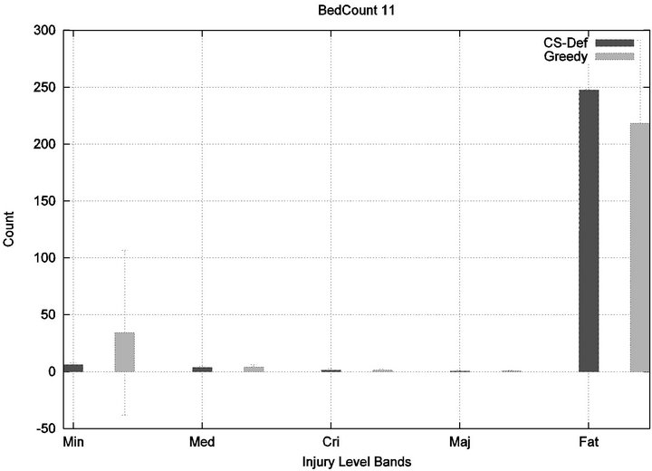 (b)
(b)
Figure 9. Greedy algorithm’s injury phase transition.
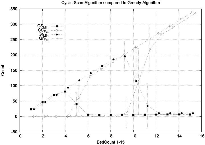
Figure 10. Tradeoffs between minor and serious injuries.
incurs injuries when the bed count exceeds 32, 10, 5, 3, for each of the scenarios. By comparison, the Cyclic Scan consistently incurs injuries whenever the bed count exceeds 8, 5, 3, 2. The ratios of these values are 4, 2, 1.6, 1.5. The experiment demonstrates that using the Greedy algorithm is able to leverage reductions in alarm treat
 (a)
(a)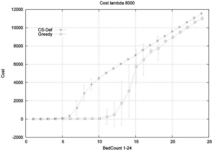 (b)
(b)
Figure 11. Exp. 1 Part 2: λ = 7.5 min and 80 min.
ment/processing time towards an increased ability to handle more patients in an injury-free manner. The conclusion is further supported by considering the upper boundaries of the phase transition where the performance of two algorithms once again coincides. This occurs at bed counts 41, 22, 7, and 3, for the four respective scenarios. The range of bed counts for which the Greedy algorithm outperforms Cyclic Scan are respectively 8 - 41, 5 - 22, 3 - 7, and 2 - 3. This shows that the Greedy algorithm’s advantage over Cyclic Scan increases in settings where treatment/processing times are lower. The graphs in Figure 14 compare the phase transitions of the Cyclic Scan and Greedy algorithms, under different assumptions for Tmax and Tfatal.
7. Experiment 2: Many Caregivers
Objective. Now we determine how the system performance curves determined in Experiment 1 are influenced by the presence of multiple caregivers. In particular, we quantify the extent to which each algorithm is able to effectively leverage the availability of additional caregivers towards healthcare delivery.
 (a)
(a)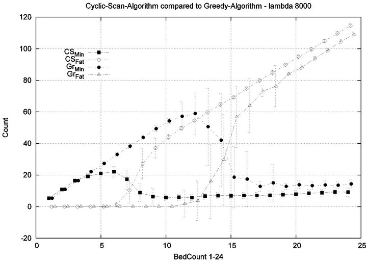 (b)
(b)
Figure 12. Exp. 1 Part 2: λ = 7.5 min and 80 min.
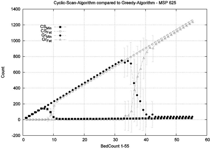
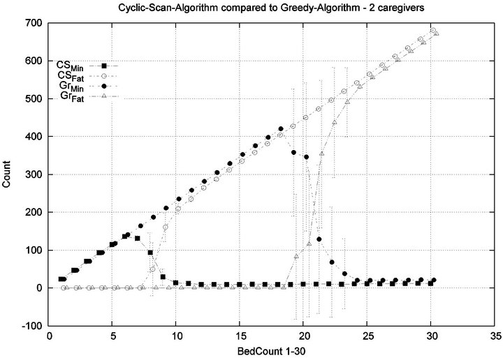
Parameters. In this experiment, we used the “baseline” configuration of Experiment 1 Part 1, but we vary the number of caregivers |C| = 1, 2, 4, 8, and we varied the bed count |P| from |C| up to 100. The graph for the 1 caregiver scenario was shown previously in Figure 7. Graphs (a), (b), (c) in Figure 15 consider the same parametrically defined baseline alarm event sequences, but submit them to critical care facilities having 2, 4, and 8 caregivers, respectively.
The Greedy algorithm incurs injuries when the bed count exceeds 8, 18, 38, 80, for each of the respective scenarios. Normalized by the number of caregivers, this sequence is 8/1 = 8, 18/2 = 9, 38/4 = 9.5, 80/8 = 10. In the Greedy scheduling system, as the number of caregivers grows, each caregiver’s contribution to the threshold value at which injuries will appear it. Informally, it pays to get more caregivers, because each new caregiver increases the effectiveness of existing caregivers. By comparison, the Cyclic Scan consistently incurs injuries whenever the bed count exceeds 4, 7, 11, 19, for each of the respective scenarios. Normalized by the number of caregivers, this sequence is 4/1 = 4, 7/2 = 3.5, 11/4 =
 (a)
(a)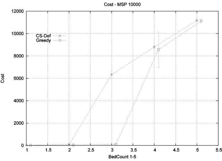 (b)
(b)
Figure 13. Exp. 1 Part 3: Tmax = 6.25 min, 100 min.
2.75, 19/8 = 2.35. In the Cyclic Scan system, as the number of caregivers grows, each caregiver’s contribution to the threshold value at which injuries decreases as well. Informally, adding more caregivers, decreases the effectiveness of existing caregivers.
We can also consider the upper boundaries of the phase transition, where the performance of two algorithms once again coincides. This occurs at bed counts 12, 24, 48, 95, for each of the respective scenarios. The intervals in which the Greedy algorithm outperforms Cyclic Scan is then 8 - 12, 18 - 24, 38 - 48, and 80 - 95 beds. The widths of these intervals are thus 4, 6, 10, and 15, for each of the respective scenarios. This in turn, indicates that the width of the interval (in terms of bed count) for which the Greedy algorithm maintains an advantage over Cyclic Scan, increases by a factor that is linear in caregiver population; doubling the number of caregivers increases the width of the interval by at least 3/2.
8. Conclusion
The current scheduling process in use in CCUs was
 (a)
(a)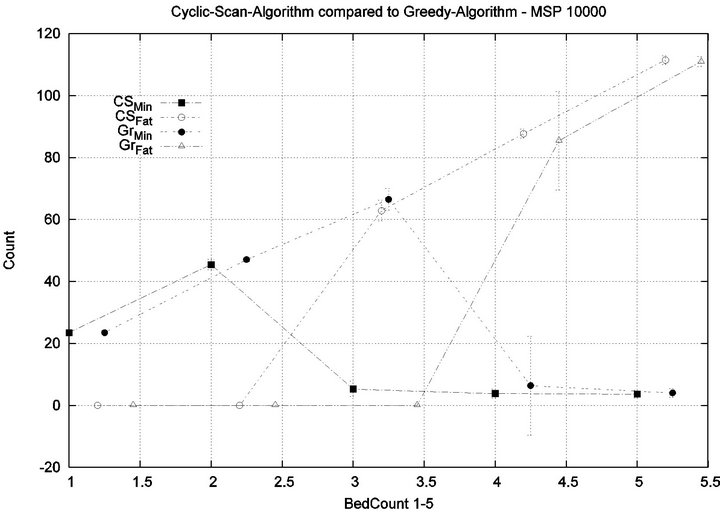 (b)
(b)
Figure 14. Exp. 1 Part 3: Tmax = 6.25 min, 100 min.
compared to a new scheduling algorithm that makes use of an (anticipated) system that integrates monitoring information (and alarms). Our simulation study provides clear evidence that such an infrastructure reduces risk to patients, and lowers operational costs. We have, through simulation, compared the defacto Cyclic Scan algorithm which caregivers follow today, against a Greedy algorithm that is only feasible at medical institutions where a vital sign data integration infrastructure is available. We have seen that such an infrastructure has the potential to yield a considerable reduction to systemic risks for patients, and significant cost reductions for healthcare providers in the number of caregivers required to adequately staff critical care facilities. These conclusions are based on compelling evidence from simulations grounded in a precise formal model: A facility that uses Greedy scheduling will make more effective use of its caregivers than the Cyclic Scan (Exp. 1, Part 1). This advantage becomes more pronounced whenever alarm frequencies drop (Exp. 1, Part 2), or treatment time decreases (Exp. 1, Part 3). In a facility using Greedy Scheduling, it pays to get more caregivers, because each new caregiver increases the
 (a)
(a)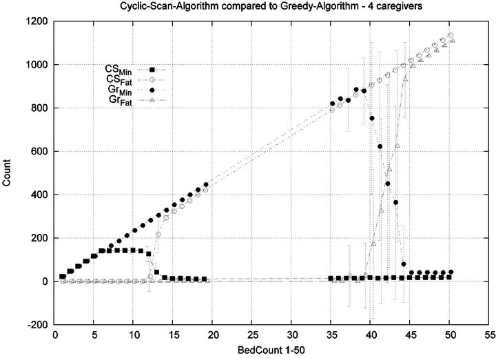 (b)
(b)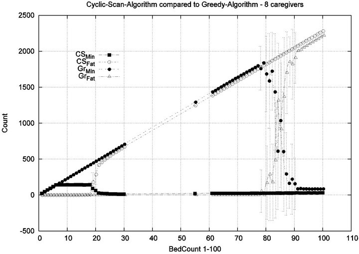 (c)
(c)
Figure 15. Experiment 2: |C| = 2, 4 and 8.
effectiveness of existing caregivers. By comparison, in a facility using Cyclic Scan, getting more caregivers, decreases the effectiveness of existing caregivers (Exp. 2). In future work, the authors intend to extend the simulation to consider algorithms which will take into account multiple vital signs with disparate injury accumulation curves. In addition, we plan to incorporate more realistic models of alarm sequences, generated by mining real historical data from vital sign streams.
REFERENCES
- J. M. Corrigan, L. T. Kohn and M. S. Donaldso, “To Err Is Human. Building a Safer Health System,” Institute of Medicine, 2000.
- S. Loughran, “In-Hospital Deaths from Medical Errors at 195,000 per Year,” Health Grades Study Finds, HealthGrades, 2004.
- The Joint Commission, “Preventing Ventilator-Related Deaths and Injuries,” Sentinel Event Alert of the Joint Commission, February 2002.
- M. McManus, M. Long, A. Cooper and E. Litvak, “Queuing Theory Accurately Models the Need for Critical Care Resources,” Anesthesiology, Vol. 100, No. 5, 2004, pp. 1271-1276. doi:10.1097/00000542-200405000-00032
- A. Zai, K. Farr, R. Grant, E. Mort, T. Ferris and H. Chueh, “Queuing Theory to Guide the Implementation of a Heart Failure Inpatient Registry Program,” Journal of American Medical Information Association, Vol. 16, No. 4, 2009, pp. 516-523. doi:10.1197/jamia.M2977
- P. Mathews, L. Drumheller and J. Carlow, “Respiratory Care Manpower Issues,” Critical Care Medicine, Vol. 34, No. 3, 2006, pp. 32-45. doi:10.1097/01.CCM.0000203103.11863.BC
- S. Gallivan, M. Utley, T. Treasure and O. Valencia, “Booked Inpatient Admissions and Hospital Capacity: Mathematical Modelling Study,” BMJ, Vol. 324, 2002, pp. 280-282. doi:10.1136/bmj.324.7332.280
- A. Shahani, S. Ridley and M. Nielsen, “Modelling Patient Flows as an Aid to Decision Making for Critical Care Capacities and Organization,” Anaesthesia, Vol. 63, No. 10, 2008, pp. 1074-1080. doi:10.1111/j.1365-2044.2008.05577.x
- G. Baskaran, A. Bargiela and R. Qu, “Hierarchical Method for Nurse Rostering Based on Granular Pre-Processing of Constraints,” Proceedings of the 23rd EUROPEAN Conference on Modelling and Simulation, Madrid, 9-12 June 2009, pp. 855-861.
- R. Ratnayaka, Z. Wang, S. Anamalamudi and S. Cheng, “Enhanced greedy optimization algorithm with data warehousing for automated nurse scheduling system,” E-Health Telecommunication Systems and Networks, Vol. 2, 2012, pp. 43-48.
- S. Kundu, M. Mahato, B. Mahanty and S. Acharyya, “Comparative performance of simulated annealing and genetic algorithm in solving nurse scheduling problem,” In Proceedings of the International MultiConference of Engineers and Computer Scientists, Hong Kong, 19-21 March 2008, p. 96.
- “JBI Clinical Online Network of Evidence for Care and Therapeutics,” The-Joanna-Briggs-Institute, Vital signs, Vol. 3, No. 3, 1999, pp. 1-6.
- K. M. Hillman, P. J. Bristow, T. Chey, K. Daffurn, T. Jacques, S. L. Norman, G. F. Bishop and G. Simmons, “Antecedents to Hospital Deaths,” Internal Medicine Journal, Vol. 31, No. 6, 2001, pp. 343-348. doi:10.1046/j.1445-5994.2001.00077.x
- J. H. Van Oostrom, C. Gravenstein and J. S. Gravenstein, “Acceptable Ranges for Vital Signs during General Anesthesia,” Journal of Clinical Monitoring and Computing, Vol. 9, 1993, pp. 321-325.
- Medical Equipment Manufacturers Directory, DRE-Inc. 2010.
- C. P. Friedman, “A Fundamental Theorem of Biomedical Informatics,” Journal of the American Medical Informatics Association, Vol. 16, No. 2, 2009, pp.169-170. doi:10.1197/jamia.M3092
- Y. B. Kim, M. Kim and Y. J. Lee, “Cosmos: A Middleware Platform for Sensor Networks and a u-Healthcare Service,” Proceedings of the 2008 ACM symposium on Applied computing, New York, 2008, pp. 512-513.
- P. Fuhrer and D. Guinard, “Building a Smart Hospital Using RFID Technologies,” European Conference on eHealth, 2006, pp. 131-142.
- S.-W. Wang, W.-H. Chen, C.-S. Ong, Li Liu, and Yun-Wen Chuang, “RFID Application in Hospitals: A Case Study on a Demonstration RFID Project in a Taiwan Hospital,” Proceedings of the 39th Annual Hawaii International Conference on System Sciences, Washington DC, 2006, p. 184.1.
- S. Manfredi, “Performance Evaluation of Healthcare Monitoring System over Heterogeneous Wireless Networks,” E-Health Telecommunication Systems and Networks, Vol. 1, pp. 27-36, 2012. doi:org/10.4236/etsn.2012.13005
- S. Czosnyka, M. Richards, H. K. Whitfield, P. Pickard, and J. Piechnik, “Cerebral Venous Blood Outflow: A Theoretical Model Based on Laboratory Simulation,” Informa Healthcare, Vol. 49, No. 5, 2001. pp. 1214-1223.
- P. W. Lai, “Model of Injury Severity Allowing for Different Gradings of Severity: Some Applications Using the British Road Accident Data,” Accident Analysis & Prevention, Vol. 12, No. 3, 1980, pp. 221-239. doi:10.1016/0001-4575(80)90023-8
- J. J. Crisco and M. M. Panjabi, “Euler stability of the human ligamentous lumbar spine. Part I: Theory,” Clinical Biomechanics, Vol. 7, No. 1, 1992, pp. 19-26. doi:10.1016/0268-0033(92)90003-M
- S. Albers and S. Leonardi, “On-Line Algorithms,” Association of Computing Machinery Computing Surveys, 1999, p. 4.
- M. Manasse, L. McGeoch and D. Sleator, “Competitive Algorithms for On-Line Problems,” Proceedings of the Twentieth Annual ACM Symposium on Theory of Computing, Chicago, 2-4 May 1988, pp. 322-333. doi:10.1145/62212.62243
NOTES
1When all vital signs share a uniform dimension, we shall for simplicity denote this common dimension as d.
2When all vital signs share a uniform dimension, we shall for simplicity denote this common dimension as d.
3Greedy selection is admittedly shortsighted, in that it focuses on alarms which have the highest risk or harm of injury at the present moment.