American Journal of Climate Change
Vol.03 No.05(2014), Article ID:52877,16 pages
10.4236/ajcc.2014.35039
Evaluation of the Eta Simulations Nested in Three Global Climate Models
Sin Chan Chou1, André Lyra1, Caroline Mourão1, Claudine Dereczynski2, Isabel Pilotto1, Jorge Gomes1, Josiane Bustamante1, Priscila Tavares1, Adan Silva1, Daniela Rodrigues1, Diego Campos1, Diego Chagas1, Gustavo Sueiro1, Gracielle Siqueira1, Paulo Nobre1, José Marengo3
1National Institute for Space Research, Cachoeira Paulista, Brazil
2Department of Meteorology, Federal University of Rio de Janeiro, Rio de Janeiro, Brazil
3Centre for Monitoring and Warning of Natural Disasters, Cachoeira Paulista, Brazil
Email: chou.sinchan@cptec.inpe.br
Copyright © 2014 by authors and Scientific Research Publishing Inc.
This work is licensed under the Creative Commons Attribution International License (CC BY).
http://creativecommons.org/licenses/by/4.0/


Received 3 September 2014; revised 5 October 2014; accepted 21 October 2014
ABSTRACT
To provide long-term simulations of climate change at higher resolution, Regional Climate Models (RCMs) are nested in global climate models (GCMs). The objective of this work is to evaluate the Eta RCM simulations driven by three global models, the HadGEM2-ES, BESM, and MIROC5, for the present period, 1961-1990. The RCM domain covers South America, Central America, and Caribbean. These simulations will be used for assessment of climate change projections in the region. Maximum temperatures are generally underestimated in the domain, in particular by MIROC5 driven simulations, in summer and winter seasons. Larger spread among the simulations was found in the minimum temperatures, which showed mixed signs of errors. The spatial correlations of temperature simulations against the CRU observations show better agreement for the MIROC5 driven simulations. The nested simulations underestimate precipitation in large areas over the continent in austral summer, whereas in winter overestimate occurs in southern Amazonia, and underestimate in southern Brazil and eastern coast of Northeast Brazil. The annual cycle of the near-surface temperature is underestimated in all model simulations, in all regions in Brazil, and in most of the year. The temperature and precipitation frequency distributions reveal that the RCM and GCM simulations contain more extreme values than the CRU observations. Evaluations of the climatic extreme indicators show that in general hot days, warm nights, and heat waves are increasing in the period, in agreement with observations. The Eta simulations driven by HadGEM2-ES show wet trends in the period, whereas the Eta driven by BESM and by MIROC5 show trends for drier conditions.
Keywords:
South America, Climate Downscaling, Model Evaluation, Climatic Extreme Indicators,
Eta Model

1. Introduction
The major tool to study future climate change is the global climate models (GCMs). To represent climate variability, these global models require having the ocean, atmosphere, and land surface in a coupled system. From the Intergovernmental Panel on Climate Change (IPCC) Fourth Assessment Report (AR4) [1] to the Fifth Assessment Report (AR5) [2] , these global models have gone through improvements and added physics complexity. In the AR5, the global models were evaluated and showed a general improvement over the AR4 models, especially in terms of precipitation, in which spatial pattern correlation increased from 0.77 to 0.82 [3] .
The AR5 GCMs start their simulations in modern industrial period, 1850, and run until 2005; from 2006 the simulations run using the Representation Concentration Pathway scenarios, generally stabilizing at 2100. To run for such a long period, grid size is a computational constraint. Generally, the resolution of coupled ocean-at- mosphere models is about 100 - 300 km. Despite the complexity of the physics processes incorporated to the latest versions of the global models, their resolutions in general may not be able to capture details of the underlying surfaces that can be important for assessment of the impacts of future climate change at local scale, for example, impacts on the urban areas, on major crop production, etc.
Regional climate model (RCM) nested to GCMs play the role of providing the details needed for local impact studies. The large-scale features are driven through the lateral boundaries. It is expected that due to resolution, the RCM may be able to improve over the driver [4] and capture more accurately the amplitude of a phenomenon [5] . The resulting climate simulated by the RCM is a combination of the climate informed by the GCM driver and its inner solution. The uncertainty through the lateral boundaries may be considered by including perturbed members of a global model as in [6] . On the other hand, [7] showed some errors shared by some RCM run over South America, driven by different GCMs. RCMs in general underestimate the precipitation and temperature over most of South America, but over the Southern parts of the Andes, it is overestimated. Temperature generally exhibited positive bias in the La Plata Basin area. These errors hint some contribution from the land-surface schemes, which are probably poorly calibrated for those regions due to the scarce observational data. In [7] different RCMs were driven by Era-Interim reanalysis [8] dataset. In this work, different three GCMs will drive the same RCM.
Prior to use the model as a tool for studying the future impacts of the simulated climate change, the model systematic errors of the present climate simulations need to be estimated so we can attribute some degree of confidence to the future climate scenarios. As part of the effort to contribute to the elaboration of the National Communication to the United Nations Framework Convention of Climate Change (UNFCCC) and to contribute to the assessment of impacts on strategic country’s issues, simulations at higher resolution were carried out using INPE (Brazilian National Institute for Space Research)’s RCM, the Eta Model. The objective of this work is to evaluate the Eta simulations nested in three GCMs: the HadGEM2-ES, BESM, and MIROC5, for the present period, 1961-1990. The period between 1961 and 1990 is chosen as present climate period so that the simulations of temperature and precipitation can have an additional comparison against the available climatology constructed by the Brazilian National Meteorological Institute [9] . The evaluation is based on mean fields, frequency distribution, and trends of climatic extreme indicators. The projections of the future climate change over South America are assessed in a companion paper [10] .
2. Data and Methodology
Three global coupled ocean-atmosphere models were considered for driving the RCM, and were taken as a minimum number of members to construct an ensemble. This poor’s man ensemble is not meant to completely encompass the uncertainty in these simulations, but to give some indication of climate conditions that model diverge or converge in their solutions. These three GCMs have distinct characteristics, which are briefly described below. An issue that rose during nesting the RCM to each global model was the length of the year. The HadGEM2-ES has 360 days in a year, MIROC5 has 365 days, and BESM has 365 + 1 in leap years. The Eta model was modified according to the global model calendar in order to assure the synchronization with the lateral boundary conditions. The RCM is described briefly following the global models’ descriptions.
The Models
1) BESM
The Brazilian Earth System Model version 2.3.1 [11] was developed by INPE. It is a spectral model with T62 truncation and 28 levels in the atmosphere. The atmosphere model is coupled to the MOM4 ocean model [12] with 50 levels in the ocean and resolution varying from 0.25 degree between 10˚N and 10˚S, 1 degree between 10˚N/S and 45˚N/S, up to 2 degree between 45˚N/S and 90˚N/S latitudes. In the longitude, the resolution is constant, 1 degree. Land-surface processes are represented by the SSiB model [13] , which distinguishes 12 types of vegetation. The sea ice uses SIS model [14] . The radiative fluxes are calculated by the CLIRAD-SW-M model [15] [16] for short wave and by Harshvardhan scheme [17] for long wave radiation. Deep convection uses Grell and Devenyi scheme [18] , whereas shallow convection uses Tiedtke scheme [19] .
2) HadGEM2-ES
The Hadley Centre Global Environmental Model [20] [21] is a grid-point model of resolution N96, which is approximately equivalent to 1.875 degrees in longitude direction and 1.275 degrees in latitude, and 38 levels in the atmosphere. In the ocean, the model has 40 levels in the vertical, and in the horizontal, the resolution varies from 1/3 degree in the tropics to 1 degree in latitudes higher than 30˚. It is a model of earth system category with representation of the carbon cycle. Over land, the carbon cycle is modelled by the dynamic vegetation TRIFFID (Top-down Representation of Interactive Foliage Including Dynamics) [22] . It distinguishes 5 plant functional types, broadleaf and needleleaf trees, C3 and C4 grass, and shrubs. The model includes atmospheric chemistry and aerosol model with organic carbon and dust representation.
3) MIROC5
MIROC5 is a Japanese cooperatively developed model known as Model for Interdisciplinary Research on Climate (MIROC), version 5 [23] . It is spectral in the atmospheric component with resolution T85, which is approximately 150 km in the horizontal, and has 40 vertical atmospheric levels. It is coupled to COCO 4.5 ocean model [24] with 50 levels in depth and 1˚ of horizontal resolution. The radiative fluxes are calculated by a k-distribution scheme [25] . The aerosol model, the SPRINTARS, is coupled to cloud microphysics scheme together with the radiation scheme, it uses the MATSIRO land surface scheme [26] with 6 soil layers. Each grid box is formed by three tiles of potential vegetation, cropland, and lake. The scheme also contains river routing and the effects of snow on albedo. Sea ice thermodynamics and dynamics are represented.
4) Eta Model
The RCM adopted for downscaling in this study is the Eta Model. This model uses the eta vertical coordinate [27] , which stays approximately horizontal in mountain areas, and which makes the coordinate suitable for studies in regions of steep topography such as the Andes Mountains in South America. This version uses a refinement, which allows sloping fluxes around the top of the mountains. The model dynamics are in finite volume [28] [29] . Deep and shallow convections are parameterized by the Betts-Miller scheme [30] modified by [31] . Cloud microphysics follow Zhao scheme [32] . The land-surface processes are represented by the NOAH scheme [33] with annual cycle of vegetation greenness. Vegetation distinguishes 12 types and soil 9 types. Radiative fluxes are treated by Lacis-Hansen scheme [34] , for short waves, and Fels-Schwarzkopf scheme [35] for long waves. CO2 is constant and kept at 330 ppm.
This model is used operationally at INPE/CPTEC since 1997 for weather forecasts [36] , since 2002 for seasonal climate forecasts [37] , and 2010 for the Brazilian Second National Communication to the UNFCCC [38] . Some evaluations carried out on the Eta model have shown the added value of its forecasts over the driver GCM forecasts [37] . A version of the Eta Model was developed for climate change studies [6] [39] [40] . This version has been validated and applied for impact and vulnerability studies [41] -[43] .
In this work, the updated version of the Eta model [29] is adapted for climate change studies and it is applied to support the Brazilian Third National Communication to the UNFCCC. The sea surface temperature is taken from the global coupled ocean models: BESM2.3.1, HadGEM2-ES, and MIROC5, and it is daily updated. Initial soil moisture and soil temperatures are derived from the global models. Lateral boundaries are updated every 6 hours. The first year of integration is discarded from the analysis. The model was set up at 20-km resolution and 38 vertical levels. Model top is set at 25 hPa. Model domain covers most of South America and Central America (Figure 1).
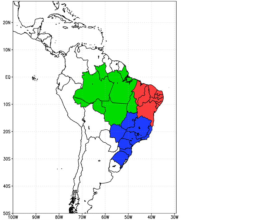
Figure 1. Model domain. Three major Brazilian regions are highlighted in the results: North (NO-green), Northeast (NE-red), and Central-South (CS- blue) Brazil.
3. Results
Model evaluation is based on comparisons between the Eta simulations and CRU [44] observations of mean values, seasonal cycle, frequency distribution, and climatic extreme indicators. The nested simulations are referred to as Eta-HadGEM2-ES, Eta-BESM, and Eta-MIROC5, when the Eta model is driven by HadGEM2-ES, BESM, and MIROC5, respectively. In order to evaluate the major climatological features, austral summer (December-January-February, DJF) and austral winter (June-July-August, JJA) seasons are examined. Results for three major Brazilian regions will be highlighted. These regions are indicated in Figure 1.
3.1. Seasonal Mean
・ Maximum and Minimum Temperatures
The maximum temperatures in DJF are simulated in Figure 2. The warmest area is simulated in the region between Paraguay and northern Argentina by the three model runs, as shown in Figures 2(a)-(c). However, a secondary maximum of temperature is simulated in the northern coast, which is not present in the observations as revealed by the errors in Figure 2(e) and Figure 2(f). Maximum temperatures in the continent are mostly underestimated, in particular by the Eta-MIROC5. Although temperatures are lower during winter, JJA (Figure 3), the errors are very similar to those errors in summer. Therefore, the maximum temperature errors are mostly related to the location than to the time of the year.
The minimum temperatures simulated in DJF show large contrast among the Eta simulation errors (Figure 4). The Eta-MIROC5 is systematically cooler than the other runs in the entire continent, whereas the Eta-BESM is

Figure 2. DJF mean maximum temperature (˚C) simulated by the downscaling: (a) Eta-HadGEM2-ES; (b) Eta-BESM; (c) Eta-MIROC5; and (d) Ensemble mean. Mean errors with respect to CRU observations for the downscaling; (e) Eta-Had- GEM2-ES; (f) Eta-BESM; (g) Eta-MIROC5; and (h) Ensemble mean error.

Figure 3. JJA mean maximum temperature (˚C) simulated by the downscaling: (a) Eta-HadGEM2-ES; (b) Eta-BESM; (c) Eta-MIROC5; and (d) Ensemble mean. Mean errors with respect to CRU observations for the downscaling; (e) Eta-Had- GEM2-ES; (f) Eta-BESM; (g) Eta-MIROC5; and (h) Ensemble mean error.
the warmest, as shown by the large area of positive bias. The positive bias of the maximum temperatures in the northern part of the continent is no longer present in the simulations of minimum temperatures, either in summer or in winter (Figure 5).

Figure 4. DJF mean minimum temperature (˚C) simulated by the downscaling: (a) Eta-HadGEM2-ES; (b) Eta-BESM; (c) Eta-MIROC5; and (d) Ensemble mean. Mean errors with respect to CRU observations for the downscaling; (e) Eta-Had- GEM2-ES; (f) Eta-BESM; (g) Eta-MIROC5; and (h) Ensemble mean error.

Figure 5. JJA mean minimum temperature (˚C) simulated by the downscaling: (a) Eta-HadGEM2-ES; (b) Eta-BESM; (c) Eta-MIROC5; and (d) Ensemble mean. Mean errors with respect to CRU observations for the downscaling; (e) Eta-Had- GEM2-ES; (f) Eta-BESM; (g) Eta-MIROC5; and (h) Ensemble mean error.
The spread of the three simulations has shown that the area that encompasses Bolivia, Paraguay, and northern Argentina is where the temperature values show generally largest disagreement, and therefore larger uncertainty.
While the biases show the location of the mean error, i.e., the deviation of the simulation with respect to the observation at each point, the general spatial pattern with the distribution of maxima and minima can be measured by the spatial correlation. Table 1 shows the spatial correlation of maximum and minimum temperatures for each three regions and the whole South America area. The ensemble of the three simulations is also evaluated. Despite the underestimate of maximum temperature in the entire continent, especially by the Eta- MIROC5 simulation, its spatial pattern is generally better positioned in DJF in comparison with the other two simulations; whereas in JJA, the Eta-HadGEM2-ES has generally higher correlation. In terms of minimum temperature, Eta-MIROC5 simulations are generally better for both seasons, DJF and JJA. The Eta-BESM exhibits the lowest correlation among the three simulations. Although the ensemble mean is expected to perform better than the individual simulations, the spatial correlation of the mean is just slightly below the highest correlation of each category.
・ Precipitation
Figure 6 and Figure 7 show the simulations of DJF and JJA mean precipitation. Precipitation in these two contrasting seasons are generally well captured by the simulations, which show the major precipitation band during DJF related to the South Atlantic Convergence Zone, and the area free of precipitation in the central and Southeast part of Brazil in JJA. In winter, the precipitation in the Southeastern South America area and the band along the eastern coast are represented in these simulations. However, in DJF the simulations show underestimate of precipitation in large areas over the continent that extends from northern Argentina to the northern part of the continent. In opposition, in JJA, the simulations show some overestimate of precipitation in the central part of the continent, in particular in southern Amazonian area. However, in JJA there remains underestimate of precipitation in the northern part, which extends over the Central America countries. In JJA, underestimate is also noticed in southern Brazil and along the eastern coast of northeast Brazil.
Over the ocean, in DJF, the Intertropical Convergence Zone (ITCZ) hints a double band over the adjacent Pacific and Atlantic Oceans. This feature is inherited from the GCMs. In JJA, the ITCZ has become a single band. The Eta-MIROC5 simulations exhibit a wider ITCZ precipitation band in both seasons. This heavier precipitation band in Eta-MIROC5 simulations extends toward the Central America and Caribbean Sea. This feature is in contrast to Eta-BESM simulations, which have little precipitation in that region in both seasons.
The spatial correlations of the mean precipitation (Table 2) show the highest values for the Eta-Had-GEM2- ES simulations for DJF, when the ensemble of the Eta simulations has shown even higher correlation with CRU observations. However, in JJA, there is no clear advantage of a single simulation or of the ensemble. In this season, the Eta-MIROC5 correlates better in NO and NE regions, whereas Eta-BESM correlates better in CS region.

Table 1. Spatial correlation between simulated seasonal mean maximum and minimum temperatures and CRU observation for DJF and JJA, for four regions: SA (South America), NO (North), NE (Northeast), CS (Centre-South of Brazil). The highest correlations are in bold.
Table 2. Spatial correlation between simulated seasonal mean precipitation and CRU observation for DJF and JJA, for four regions: SA (South America), NO (North), NE (Northeast), CS (Centre-South of Brazil). The highest correlations are in bold.
![]()
Figure 6. DJF mean precipitation (mm/day) simulated by the downscaling: (a) Eta-HadGEM2-ES; (b) Eta-BESM; (c) Eta- MIROC5; and (d) Ensemble mean. Mean errors with respect to CRU observations for the downscaling; (e) Eta-Had-GEM2- ES; (f) Eta-BESM; (g) Eta-MIROC5; and (h) Ensemble mean error.
3.2. Annual Cycle
The annual cycle of near-surface temperature (Figure 8) is underestimated in simulations, either by the regional or by the global models, in all three Brazilian regions, and in most time of the year. Nevertheless, the error of the nested simulations does not exhibit the same pattern with respect to the driver global model errors. For example, the Eta-HadGEM2-ES simulations are warmer than HadGEM2-ES in the CS region and during winter in the NO region. While the Eta-MIROC5 simulations are systematically colder than MIROC5, the Eta-BESM simulations are systematically warmer than BESM in all three regions. Therefore, the nested simulations did not reveal a regular pattern of error with respect to the driver global model. The BESM surface temperature may be systematically colder in all regions as it represents the first model layer, which has 60 m of depth and not at 2 m of height as other model near-surface temperature.
The annual cycle of precipitation (Figure 9) simulated by the Eta model is generally smaller than the respective driver global models precipitation, especially during the rainy season, DJF. This causes the Eta simulations to reproduce a better annual cycle of precipitation in CS and NE regions, where global model precipitation is excessive during rainy period. In NO region, precipitation is largely underestimated by the regional model. During winter (JJA) in CS, while the global models tend to underestimate the precipitation, the regional simulations
![]()
Figure 7. JJA mean precipitation (mm/day) simulated by the downscaling: (a) Eta-HadGEM2-ES; (b) Eta-BESM; (c) Eta- MIROC5; and (d) Ensemble mean. Mean errors with respect to CRU observations for the downscaling: (e) Eta-Had- GEM2-ES; (f) Eta-BESM; (g) Eta-MIROC5; and (h) ensemble mean error.
![]() (a) (b) (c)
(a) (b) (c)
Figure 8. Mean annual cycle of temperature (˚C) simulated by the regional and global models, and CRU observations, for the three regions: (a) NO; (b) NE and (c) CS. The Eta simulations are in solid lines and the global model simulations are in dashed lines. Observations are in solid black.
overestimate it. The ensemble of the Eta simulations follows closer the CRU observed annual cycle in NE and CS regions, whereas in the NO region, the global model ensemble precipitation follows closer to the CRU observations.
3.3. Frequency Distribution
The distributions of monthly temperatures in the major three regions (Figure 10) shows that model simulations reach more extreme values than the monthly CRU observations, although of very small frequency. The frequency is shown logarithmicax is to allow displaying the low frequency in the extreme value ranges. Therefore, the ensemble of model temperatures produces a broader distribution. The feature of narrower distribution in the NO and NE regions, due to small temperature variability in the tropics, is captured by the Eta simulations, as well as the broader distribution in the subtropical CS region. In general, the Eta-MIROC5 produces a distribu-
![]()
Figure 9. Mean annual cycle of precipitation (mm/day) simulated by the regional and global models, and CRU observations, for the three regions: (a) NO; (b) NE and (c) CS. The Eta simulations are in solid lines and the global model simulations are in dashed lines. Observations are in solid black.
![]()
Figure 10. Frequency distribution (%) of monthly temperatures (˚C) for the period 1961-1990, for the regions (a) NO, (b) NE, and (c) CS of Brazil, for RCM and GCM simulations, and the respective ensemble mean values. The CRU observations are indicated in solid black curve. Frequency axis is logarithmic.
tion of temperatures lower than its driver global model, whereas the Eta-BESM produces a distribution of temperatures warmer than the BESM. In the case of Eta-HadGEM2-ES, there are mixed results in the three regions. The peaks at the most frequent values are generally displaced in the simulations by about 2˚C to 4˚C. Errors in the distribution of temperature are generally related to the models’ land-surface representations. A source of uncertainty in the distribution of the CRU observations is due to the poor distribution of actual observations in Brazil, mostly in the regions such as of complex topography, or in forest of difficult access. In these areas model simulations will produce values, but observations are never recorded.
Similar to temperatures, the monthly precipitation simulated by the models tends to reach larger amounts than the recorded by the CRU observations (Figure 11). In particular, the downscaling simulations can produce daily heavier precipitation that accumulates to larger amounts in a monthly total, which occurs in all three regions. In general, the models capture the peaks of most frequent monthly precipitation values, which occur in the range of 1 - 9 mm/day. Toward larger precipitation rates, the observations display a linear-log distribution, which is generally captured by the Eta model simulations, with some variations of the slope among the three different regions. The simulated precipitation amount is mostly dependent on individual model convection and cloud schemes. The Eta precipitation distributions do not follow the global model distribution curves or slopes. For example, in CS region, where the Eta-BESM reaches extreme precipitation rates, BESM simulations do not exceed the rate of 13 mm/day; or the opposite case in NO region, where Eta-BESM simulations do not exceed 33 mm/day, and BESM exceeds 41 mm/day. Therefore, the Eta precipitation distributions in all three regions depart from the driver model distributions, but the downscaling distributions still exhibit spread among their members. The uncertainty of the observations mentioned for the temperature values is also valid for the precipitation observations.
![]()
Figure 11. Frequency distribution (%) of monthly precipitation (mm/day) for the period 1961-1990, for the regions (a) NO, (b) NE, and (c) CS of Brazil, for regional and global model simulations, and the respective models ensemble mean values. The CRU observations are indicated in solid black curve. Frequency axis is logarithmic.
3.4. Climatic Extreme Indicators
Figure 12 shows the linear trends of some climatic extreme indicators [45] derived for temperatures, such as the 90th percentile of maximum temperatures or warm days (TX90p), the 90th percentile of minimum temperatures or warm nights (TN90p), and the consecutive days, greater than 6 days, of temperature above the 90th percentile which is equivalent to heat waves (Warm Spell Duration Indicator-WSDI). The climatic extreme indicators derived for precipitation (Figure 13) are the total annual rainfall PRCPTOT, the maximum annual rainfall on five consecutive days (RX5Day), the annual mount of rainfall falling above the 95th percentile (R95p), the maximum number of consecutive wet days in the year (CWD) and the maximum number of consecutive dry days in the year (CDD).
Observational studies on temperature extremes over South America show a general warming in the region [46] -[49] . In [47] , the largest warming trends were observed over northeastern Brazil with decrease of cold nights and increase of warm nights. That work also found the second largest warming trends in the Amazon region for both indicators, whereas heat waves increased significantly over Northeast Brazil (approximately 11 days longer), the Amazon, and the western South America. In these simulations, the Eta-HadGEM2-ES and Eta- BESM simulations show increasing trends of TX90p, TN90p and WSDI in agreement with observational studies. However, the largest warming areas in these simulations occur in the northern part of the continent, not in Northeast of Brazil as suggested by those observational studies. The Eta-MIROC5 simulations show temperature indicator trends opposite to the other model simulations. The decrease trends in temperature extreme indicators in Eta-MIROC5 occur due to the period chosen for the trend. After 1990, the trend turns to positive toward 2005 and beyond in the transient period.
Reference [50] showed that for southern Brazil, Uruguay, northern and central Argentina, as well as in northern Peru and Ecuador trends are toward a wetter climate in the period 1960-2000, while in southern Peru and southern Chile there is a tendency toward a drier climate. This is in agreement with [47] who found that the total annual precipitation over the South America is approximately 92 mm higher in the present day than in 1950, with increase of heavy rainfall events. Precipitation indicators show opposite trends between Eta-HadGEM2-ES simulation and the other two model simulations, the Eta-MIROC5, and the Eta-BESM. The Eta-HadGEM2-ES simulations show wet trends in the period 1961-1990, over most of South America, as suggested by the increase in the PRCPTOT, RX5DAY, R95p, and CWD and decrease in CDD. Only in the northeastern South America and in northern Chile, the Eta-HadGEM2-ES simulation displays trends for drier conditions in the period. In contrast, the Eta-MIROC5 and Eta-BESM simulations in general display trends for drier conditions over most of South America, especially in the northern part of the continent. However, some patchy areas of increase of precipitation are found in southeastern South America in these two simulations. In northeast of Brazil, while the Eta-BESM simulations show increase of annual precipitation (PRCPTOT) in most of the region, the Eta-MIROC5 simulations show mostly decrease which agrees with the trend in three stations shown by [47] . For CWD, [49] have found this indicator increasing in the southeastern South America reaching about 12 days, whereas the Eta-HadGEM2-ES and Eta-MIROC5 have CWD increasing in a narrower area of southeast of Brazil. The de-
![]()
Figure 12. Trends of climatic extreme indicators in the period 1961-1990 of. (a)-(c) 90th percentile of maximum temperature (TX90p); (d)-(f) 90th percentile of minimum temperature (TN90p); (g)-(i) Consecutive days, greater than 6 days, of temperature above the 90th percentile (WSDI). Eta-HadGEM2-ES trends are in the left, Eta-BESM are in the middle, and Eta- MIROC5 are in the right column.
cline of CDD in central and southern part of Brazil, Uruguay, and Paraguay observed in the work [49] is somehow captured by Eta-HadGEM2-ES.
4. Conclusions
The Eta RCM nested in three GCMs reproduces a 30-year present climate period. The global models adopted to drive the RCM are the HadGEM2-ES, MIROC5, and the BESM. Synchronicity and compatibility with the driver conditions were taken into account in the nested simulations. The evaluation of the present period, 1961-1990
![]()
![]()
Figure 13. Trends of climatic extreme indicators in the period 1961-1990 of (a)-(c) annual total precipitation (PRCPTOT); (d)-(f) annual maximum 5-day accumulated precipitation (RX5DAY); (g)-(i) 95th percentile of daily precipitation (R95p); (j)-(l) maximum annual consecutive dry days (CDD); (m,n,o) maximum annual consecutive wet days (CWD). Eta-Had- GEM2-ES trends are in the left, Eta-BESM are in the middle, and Eta-MIROC5 are in the right column.
against CRU observations shows that the Eta simulations generally reproduces the general climatological features over the South America continent.
Temperature is generally underestimated in the Eta simulations. This is shown in the spatial distribution and the mean annual cycle. However, simulations show large negative bias of precipitation in the North region of Brazil during summer, and positive bias in southern part of NO in winter. The source of this error requires further investigation, through either the cumulus convection or the land-surface representation parameterization schemes. Some error features are inherited from the global models, such as the double precipitation band of the ITCZ. Model bias over mountains area, either for temperature or precipitation, is still uncertain due to the scarce observations over those areas. Frequency distribution reveals that the RCM and GCM simulations exhibit more extreme values of monthly values of temperature and precipitation than the CRU observations. Despite the errors shown in this evaluation, the nested simulations contain the major features of the South America and Central America climatology.
Acknowledgements
The authors thank: the Brazilian Ministry of Science, Technology, and Innovation for supporting the work through Global Environmental Facility funding (UNDP BRA/05/G31), the Secretariat for Strategic Affairs of the presidency of Brazil for additional funding, Martin Juckes from the British Atmospheric Data Centre for making available HadGEM2-ES dataset, and Seita Emori and Tokuta Yokohata from the National Institute for Environmental Studies for making available the MIROC5 dataset. S.C.C. thanks the Brazilian National Council for Scientific and Technological Development for the grant PQ 308035/2013-5.
References
- IPCC (2007) Climate Change 2007: The Physical Science Basis. Contribution of Working Group I to the Fourth Assessment Report of the Intergovernmental Panel on Climate Change. Solomon, S., Qin, D., Manning, M., Chen, Z., Marquis, M., Averyt, K.B., Tignor, M. and Miller, H.L., Eds., Cambridge University Press, Cambridge, United Kingdom and New York, 996.
- IPCC (2013) Climate Change 2013: The Physical Science Basis. Contribution of Working Group I to the Fifth Assessment Report of the Intergovernmental Panel on Climate Change. Stocker, T.F., Qin, D., Plattner, G.-K., Tignor, M., Allen, S.K., Boschung, J., Nauels, A., Xia, Y., Bex, V. and Midgley, P.M., Eds., Cambridge University Press, Cambridge, United Kingdom and New York, 1535. http://dx.doi.org/10.1017/CBO9781107415324
- Flato, G., Marotzke, J., Abiodun, B., Braconnot, P., Chou, S.C., Collins, W., Cox, P., Driouech, F., Emori, S., Eyring, V., Forest, C., Gleckler, P., Guilyardi, E., Jakob, C., Kattsov, V., Reason, C. and Rummukainen, M. (2013) The Physical Science Basis. Contribution of Working Group I to the Fifth Assessment Report of the Intergovernmental Panel on Climate Change. Stocker, T.F., Qin, D., Plattner, G.-K., Tignor, M., Allen, S.K., Boschung, J., Nauels, A., Xia, Y., Bex, V. and Midgley, P.M., Eds., Cambridge University Press, Cambridge, United Kingdom and New York, Chapter 9, 741-866. http://dx.doi.org/10.1017/CBO9781107415324.020
- Veljovic, K., Rajkovic, B., Fennessy, M.J., Altshuler, E.L. and Mesinger, F. (2010) Regional Climate Modeling: Should One Attempt Improving on the Large Scales? Lateral Boundary Condition Scheme: Any Impact? Meteor Zeitschrift, 19, 237-246. http://dx.doi.org/10.1127/0941-2948/2010/0460
- Laprise, R., de Elía, R., Caya, D., et al. (2008) Challenging Some Tenets of Regional Climate Modelling. Meteoroly and Atmospheric Physics, 100, 3-22. http://dx.doi.org/10.1007/s00703-008-0292-9
- Chou, S.C., Marengo, J.A., Lyra, A.A., et al. (2012) Downscaling of South America Present Climate Driven by 4- Member HadCM3 Runs. Climate Dynamics, 38, 635-653. http://dx.doi.org/10.1007/s00382-011-1002-8
- Solman, S.A., Sanchez, E., Samuelsson, P., et al. (2013) Evaluation of an Ensemble of Regional Climate Model Simulations over South America Driven by the ERA-Interim Reanalysis: Model Performance and Uncertainties. Climate Dynamics, 41, 1139-1157. http://dx.doi.org/10.1007/s00382-013-1667-2
- Simmons, A., Uppala, S., Dee, D. and Kobayashi, S. (2007) ERA-Interim: New ECMWF Reanalysis Products from 1989 Onwards. ECMWF News, 110, 25-35.
- INMET (2009) Normais Climatológicas do Brasil (1961-1990) Reeditado e Ampliado, organizadores: Andrea Malheiros Ramos, Luiz André Rodrigues dos Santos, Lauro Tadeu Guimarães Fortes. Brasília, DF, 465 p.
- Chou, S.C., Lyra, A., Mourão, C., Dereczynski, C., Pilotto, I., Gomes, J., Bustamante, J., Tavares, P., et al. (2014) Assessment of Climate Change over South America under RCP 4.5 and 8.5 Downscaling Scenarios. American Journal of Climate Change.
- Nobre, P., Siqueira, L.S.P., de Almeida, R.A.F., Malagutti, M., Giarolla, E., Castelão, G.P., et al. (2013) Climate Simulation and Change in the Brazilian Climate Model. Journal of Climate, 26, 6716-6732. http://dx.doi.org/10.1175/JCLI-D-12-00580.1
- Griffies, S.M. (2009) Elements of MOM4p1. NOAA/Geophysical Fluid Dynamics Laboratory Ocean Group Technical Report No. 6, 444.
- Xue, Y., Sellers, P.J., Kinter, J.L. and Shukla, J. (1991) A Simplified Biosphere Model for Global Climate Studies. Journal of Climate, 4, 345-364. http://dx.doi.org/10.1175/1520-0442(1991)004<0345:ASBMFG>2.0.CO;2
- Winton, M. (2000) A Reformulated Three-Layer Sea Ice Model. Journal of Atmospheric and Oceanic Technology, 17, 525-531. http://dx.doi.org/10.1175/1520-0426(2000)017<0525:ARTLSI>2.0.CO;2
- Tarasova, T.A., Barbosa, H.M.J. and Figueroa, S.N. (2006) Incorporation of New Solar Radiation Scheme into CPTEC GCM. Instituto Nacional de Pesquisas Espaciais Technical Report, INPE-14052-NTE/371, 44.
- Chou, M.D. and Suarez, M.J. (1999) A Solar Radiation Parameterization (CLIRAD-SW) for Atmospheric Studies. NASA Tech. Memo NASA/TM-1999-104606, 40.
- Harshvardhan, Davies, R., Randall, D.A. and Corsetti, T.G. (1987) A Fast Radiation Parameterization for General Circulation Models. Journal of Geophysical Research, 92, 1009-1016. http://dx.doi.org/10.1029/JD092iD01p01009
- Grell, G.A. and Devenyi, D. (2002) A Generalized Approachto Parameterizing Convection Combining Ensemble and Data Assimilation Techniques. Geophysical Research Letters, 29, 38-1-38-4.
- Tiedtke, M. (1984) The Sensitivity of the Time Mean Large-Scale Flow to Cumulus Convection in the ECMWF Model. Workshop on Convection in Large-Scale Numerical Models, Reading, United Kingdom, ECMWF, 297-316.
- Collins, W.J., Bellouin, N., Doutriaux-Boucher, M., Gedney, N., Halloran, P., Hinton, T., et al. (2011) Development and Evaluation of an Earth-System Model-HadGEM2. Geoscientific Model Development, 4, 1051-1075. http://dx.doi.org/10.5194/gmd-4-1051-2011
- Martin, G.M., Bellouin, N., Collins, W.J., Culverwell, I.D., Halloran, P.R., Hardiman, S.C., et al. (2011) The HadGEM2 Family of Met Office Unified Model Climate Configurations. Geoscientific Model Development, 4, 723-757. http://dx.doi.org/10.5194/gmd-4-723-2011
- Cox, P.M. (2001) Description of the “TRIFFID” Dynamic Global Vegetation Model. Hadley Centre Technical Note 24, Met Office, UK.
- Watanabe, M., Suzuki, T., O’ishi, R., Komuro, Y., Watanabe, S., Emori, S., et al. (2010) Improved Climate Simulation by MIROC5: Mean States, Variability, and Climate Sensitivity. Journal of Climate, 23, 6312-6335. http://dx.doi.org/10.1175/2010JCLI3679.1
- Hasumi, H. (2007) CCSR Ocean Component Model (COCO), Version 4.0. CCSR Report, Centre for Climate System Research.
- Sekiguchi, M. and Nakajim, T. (2008) A k-Distribution-Based Radiation Code and Its Computational Optimization for an Atmospheric General Circulation Model. Journal of Quantitative Spectroscopy and Radiative Transfer, 109, 2779- 2793. http://dx.doi.org/10.1016/j.jqsrt.2008.07.013
- Takata, K., Emori, S. and Watanabe, T. (2003) Development of the Minimal Advanced Treatments of Surface Interaction and Runoff. Global and Planetary Change, 38, 209-222. http://dx.doi.org/10.1016/S0921-8181(03)00030-4
- Mesinger, F. (1984) A Blocking Technique for Representation of Mountains in Atmospheric Models. Rivista di Meteorologia Aeronautica, 44, 195-202.
- Janjić, Z.I. (1984) Nonlinear Advection Schemes and Energy Cascade on Semi-Staggered Grids. Monthly Weather Review, 112, 1234-1245. http://dx.doi.org/10.1175/1520-0493(1984)112<1234:NASAEC>2.0.CO;2
- Mesinger, F., Chou, S.C., Gomes, J.L., Jovic, D., Bastos, P., Bustamante, J.F., et al. (2012) An Upgraded Version of the Eta Model. Meteorology and Atmospheric Physics, 116, 63-79. http://dx.doi.org/10.1007/s00703-012-0182-z
- Betts, A.K. and Miller, M.J. (1986) A New Convective Adjustment Scheme. Part II: Single Column Tests Using GATE Wave, BOMEX, ATEX and Arctic Air-Mass Data Sets. Quarterly Journal of the Royal Meteorological Society, 112, 693-709.
- Janjić, Z.I. (1994) The Step-Mountain Eta Coordinate Model: Further Developments of the Convection, Viscous Sublayer, and Turbulence Closure Schemes. Monthly Weather Review, 122, 927-945. http://dx.doi.org/10.1175/1520-0493(1994)122<0927:TSMECM>2.0.CO;2
- Zhao, Q., Black, T.L. and Baldwin, M.E. (1997) Implementation of the Cloud Prediction Scheme in the Eta Model at NCEP. Weather and Forecasting, 12, 697-712. http://dx.doi.org/10.1175/1520-0434(1997)012<0697:IOTCPS>2.0.CO;2
- Ek, M., Mitchell, K.E., Lin, Y., Rogers, E., Grunmann, P., Koren, V., Gayno, G. and Tarpley, J.D. (2003) Implementation of Noah Land Surface Model Advances in the National Centers for Environmental Prediction Operational Mesoscale Eta Model. Journal of Geophysical Research, 108, 8851. http://dx.doi.org/10.1029/2002JD003296
- Lacis, A.A. and Hansen, J. (1974) A Parameterization for the Absorption of Solar Radiation in the Earth’s Atmosphere. Journal of the Atmospheric Sciences, 31, 118-133. http://dx.doi.org/10.1175/1520-0469(1974)031<0118:APFTAO>2.0.CO;2
- Fels, S.B. and Schwarzkopf, M.D. (1975) The Simplified Exchange Approximation: A New Method for Radiative Transfer Calculations. Journal of the Atmospheric Sciences, 32, 1475-1488. http://dx.doi.org/10.1175/1520-0469(1975)032<1475:TSEAAN>2.0.CO;2
- Chou, S.C. (1996) Modelo Regional Eta. Climanálise. Vol. 1, Especial Edition, Instituto Nacional de Pesquisas Espaciais, São José dos Campos.
- Chou, S.C., Bustamante, J.F. and Gomes, J.L. (2005) Evaluation of Eta Model Seasonal Precipitation Forecasts over South America. Nonlinear Processes in Geophysics, 12, 537-555. http://dx.doi.org/10.5194/npg-12-537-2005
- MCT (2010) Second National Communication of Brazil to the United Nations Framework Convention on Climate Change. Ministério da Ciência e Tecnologia, Brasília.
- Pesquero, J.F., Chou, S.C., Nobre, C.A. and Marengo, J.A. (2009) Climate Downscaling over South America for 1961-1970 Using the Eta Model. Theoretical and Applied Climatology, 99, 75-93. http://dx.doi.org/10.1007/s00704-009-0123-z
- Marengo, J.A., Chou, S.C., Kay, G., Alves, L.M., Pesquero, J.F., Soares, W.R., et al. (2012) Development of Regional Future Climate Change Scenarios in South America Using the Eta CPTEC/HadCM3 Climate Change Projections: Climatology and Regional Analyses for the Amazon, São Francisco and the Parana River Basins. Climate Dynamics, 38, 1829-1848. http://dx.doi.org/10.1007/s00382-011-1155-5
- Matos, A.C., Dereczynski, C.P., Chou, S.C. and Palmeira, R. (2012) Investigação do comportamento dos ciclones no clima futuro a partir do modelo regional Eta-HadCM3. Anais do XVII Congresso Brasileiro de Meteorologia, Gramado, RS, September, 2012, 1-5.
- Resende, N.C., Giarolla, A., Rodrigues, D.C., Tavares, P. and Chou, S.C. (2011) Ocorrência da doença ferrugem-do- café (Hemileia vastatrix) em algumas regiões de São Paulo, baseada nas projeções climáticas do modelo Eta/CPTEC (Cenário A1B-IPCC/SRES). XVII Congresso Brasileiro de Agrometeorologia, Guarapari-ES, July 2011, 1.
- Rodrigues, D.C., Tavares, P., Giarolla, A., Chou, S.C., Resende, N.C. and De Camargo, M.B.P. (2011) Estimativa da ocorrência de temperatura máximamaior que 34˚C durante o florescimento e maturação do cafeeiro baseado no modelo Eta/CPTEC 40km (cenário A1B). XVII Congresso Brasileiro de Agrometeorologia, Guarapari-ES, July 2011, 1.
- Mitchell, T.D. and Jones, P.D. (2005) An Improved Method of Constructing a Database of Monthly Climate Observations and Associated High-Resolution Grids. International Journal of Climatology, 25, 693-712. http://dx.doi.org/10.1002/joc.1181
- Frich, P., Alexander, L.V., Della-Marta, P., Gleason, B., Haylock, M., Klein Tank, A.M.G. and Peterson, T. (2002) Observed Coherent Changes in Climatic Extremes during the Second Half of the Twentieth Century. Climate Research, 19, 193-212. http://dx.doi.org/10.3354/cr019193
- Vincent, L.A., Peterson, T.C., Barros, V.R., Marino, M.B., Rusticucci, M., Carrasco, G., et al. (2005) Observed Trends in Indices of Daily Temperature Extremes in South America 1960-2000. Journal of Climate, 18, 5011-5023. http://dx.doi.org/10.1175/JCLI3589.1
- Skansi, M.M., Brunet, M., Sigró, J., Aguilar, E., Arevalo Groening, J.A., Bentancur, O.J., et al. (2013) Warming and Wetting Signals Emerging from Analysis of Changes in Climate Extreme Indices over South America. Global and Planetary Change, 100, 295-307. http://dx.doi.org/10.1016/j.gloplacha.2012.11.004
- Alexander, L.V., Zhang, X., Peterson, T.C., Caesar, J., Gleason, B., Klein Tank, A.M.G., et al. (2006) Global Observed Changes in Daily Climate Extremes of Temperature and Precipitation. Journal of Geophysical Research, 111, Article ID: D05109. http://dx.doi.org/10.1029/2005JD006290
- Marengo, J.A., Rusticucci, M., Penalba, O. and Renom, M. (2010) An Intercomparison of Observed and Simulated Extreme Rainfall and Temperature Events during the Last Half of the Twentieth Century: Part 2: Historical Trends. Climatic Change, 98, 509-529. http://dx.doi.org/10.1007/s10584-009-9743-7
- Haylock, M.R., Peterson, T.C., Alves, L.M., Ambrizzi, T., Anunciação, Y.M.T., Baez, J., et al. (2006) Trends in Total and Extreme South American Rainfall in 1960-2000 and Links with Sea Surface Temperature. Journal of Climate, 19, 1490-1512. http://dx.doi.org/10.1175/JCLI3695.1