American Journal of Climate Change
Vol. 2 No. 3A (2013) , Article ID: 37301 , 13 pages DOI:10.4236/ajcc.2013.23A003
Spanish Extreme Winds and Their Relationships with Atlantic Large-Scale Atmospheric Patterns
1Dpto. Astrofísica y CC. Física de la Atmósfera, Facultad de CC Físicas, Universidad Complutense de Madrid, Ciudad Universitaria, Madrid, Spain
2Dpto. Matemática Aplicada, Escuela Universitaria de Informática, Universidad de Valladolid, Segovia, Spain
3Agencia Estatal de Meteorología, C/Leonardo Prieto Castro, Madrid, Spain
Email: a.depascual@fis.ucm.es, valero@fis.ucm.es, mlmartin@eii.uva.es, cgarcialegaz@aemet.es
Copyright © 2013 Alvaro Pascual et al. This is an open access article distributed under the Creative Commons Attribution License, which permits unrestricted use, distribution, and reproduction in any medium, provided the original work is properly cited.
Received May 29, 2013; revised June 28, 2013; accepted July 24, 2013
Keywords: Extreme Winds; Gusts; Atmospheric Circulation Variability; Analogs; Probabilistic Results
ABSTRACT
The purpose of this work is to review procedures to obtain relationships between wind and large-scale atmospheric fields, with special emphasis on extreme situation results. Such relationships are obtained by using different methods and techniques such as wind cumulative probability functions and composite maps. The analyses showed different mean atmospheric situations associated with the different wind patterns, in which strong atmospheric gradients can be related to moderate to strong winds in Spain. Additionally, a statistical downscaling analog model, developed by the authors, is used for diagnosing large-scale atmospheric circulation patterns and subsequently estimating extreme wind probabilities. From an atmospheric circulation pattern set obtained by multivariate methodology applied to a large-scale atmospheric circulation field, estimations of wind fields, particularly extreme winds, are obtained by means of the analogs methodology. Deterministic and probabilistic results show that gust behaviour is quite better approximated than mean wind speed, in general. The model presents some underestimations except for strong winds. Moreover, the model shows better probabilistic wind results over the Spanish northern area, highlighting that the atmospheric situations coming from the Atlantic Ocean are better recovered to predict mean wind and gusts in the Northern Peninsula.
1. Introduction
Winter storms are responsible for more than 50% of the total economic loss in central Europe, due to natural hazards [1,2] and a single extreme storm event can cause economic losses exceeding 10 billion euros. A rise in storm-related monetary losses for Europe in the course of the 20th century has been observed by Barredo [3], explained principally by changes in economic and demographic conditions, with much of the recent infrastructure in various parts of the world increasingly constructed in zones at risk from severe weather [2]. Therefore, the knowledge of atmospheric circulation patterns, particularly the one dealing with atmospheric patterns conducive to risky meteorological situations related to extreme wind events, is especially important for wind energy applications [4-6]. Forecasters, energy producers and grid operators have different views on what extremes related to wind generation are. Extreme events have been categorized taken into account damages and economic loss
[7,8]. Extremes have been also identified as their occurrence probabilities [9]; they have been analyzed from the spatial-temporal characteristics of prediction errors [10], or taking into account their probabilistic forecasts by statistical scenarios [11,12], by ensemble predictions [13]. The final analysis can be used for nowcasting wind power over the whole area, and for data assimilation purposes (in order to update and improve wind power predictions) for better understanding the, or for issuing “global” warnings related to expected accuracy of weather and wind power forecasts over the area considered.
In determining temporal-spatial distribution changes of wind and other climatological elements, it is necessary to take into account the atmospheric circulation variability. The Western European climate steps are necessary on the available knowledge of natural variability in regional scales and its relationship to large-scale circulation [14- 20]. The relative location of different pressure centers over the North Atlantic area influence different air masses with distinct physical characteristics over Iberia to produce a wide range of differentiated regional climates, playing the topography a leading role. In fact, at local scales the development of cloud systems or the enhancement of wind speed over different areas can be especially affected due to the topography [21-23]; at largescale domains, topography can generate o redirected synoptic and mesoscale flows [24]. The present study is firstly focused on showing relationships between wind and large-scale atmospheric fields over an Atlantic area, with special emphasis on results involving extreme situations. These connections are attained by using different methods and procedures, such us cumulative probability curves and composite maps. Composites have already been used by the authors in several studies in order to analyse different fields, obtaining relationships between them, so that maximum and minimum intensity phases of a field can be related to the other one [16,18,19].
On the other hand, the improvement of meteorological forecasts of wind by means of dynamic modelling has been progressing by means of limited area models or ensemble prediction systems in several research projects (ANEMOS, ANEMOS.plus). However, this methodology bears high computational costs. In order to overcome this problem, the analog method for predicting time series can be used [25]. With this method, local prediction models are obtained finding in a set of historic data similar situations to a particular situation [26-28]. This technique has been implemented for both climatic anomaly predictions [29,30] and short-range prediction [31], revealing as an alternative to other more complex models with high computational cost. In the framework of the European Project SafeWind, the authors have been developing several works based on multivariate methodologies for obtaining atmospheric situations analog to a situation associated with extreme winds [32]. One of the final purposes of this European Project is to develop a statistical downscaling model (ANPAF: ANalog PAttern Finder) for diagnosing large-scale atmospheric circulation patterns and subsequently estimating extreme wind probabilities. In the present paper, from an atmospheric circulation pattern set obtained by multivariate methodology [18,19,33,34] applied to a large-scale atmospheric circulation field, estimations of wind fields, particularly extreme winds, are obtained by means of the analogs methodology.
The study is organized as follows. In Section 2, data used in the study are described. In Section 3, the connections between wind speeds and large-scale atmospheric patterns are shown, presenting the relationships between large-scale atmospheric patterns and wind speed patterns statistically obtained. Moreover, the interactions between observational winds and large-scale atmospheric circulation statistical modes are provided and analyzed. Section 4 is devoted to analyze the analog results for both the large-scale atmospheric field and the Spanish mean wind speed and wind gust, in terms of some deterministic and probabilistic tools. The main conclusions are drawn in Section 5.
2. Data
In order to analyze the relationships between wind speeds and large-scale atmospheric fields and to extract information about extreme situations it is very important to select the appropriate datasets. In this work, in order to characterize the atmospheric circulation, 1000 hPa daily geopotential heights at 12:00 UTC (Z1000) for 36 winters from 1971 to 2007 covering from 51.5˚W to 15.5˚E and 20˚ to 60˚N have been used. Z1000 data are a product of the ERA40 Reanalysis [35]. Concerning the wind speed, firstly daily mean wind speed (MWS) data for 21 stations distributed over Spain (Figure 1) during the winter (D-J-F) season from 1970 to 2002 have been considered. These wind data come from in-situ measurements of the station network of the Spanish Meteorological Service (Agencia Estatal de Meteorología, AEMET). In order to analyze the relationships between wind speeds and large-scale atmospheric fields and to extract information about extreme situations it is very important to select the appropriate datasets. In this work, in order to characterize the atmospheric circulation, 1000 hPa daily geopotential heights at 12:00 UTC (Z1000) for 36 winters from 1971 to 2007 covering from 51.5˚W to 15.5˚E and 20˚ to 60˚N have been used. Z1000 data are a product of the ERA40 Reanalysis [35]. Concerning the wind speed, firstly daily mean wind speed (MWS) data for 21 stations distributed over Spain (Figure 1) during the winter (D-J-F) season from 1970 to 2002 have been considered. These wind data come from in-situ measurements of the station network of the Spanish Meteorological Service (Agencia Estatal de Meteorología, AEMET).
On the other hand, some techniques for estimating and forecasting wind speeds are reviewed, with special emphasis in extreme winds. To do this wind speed and wind gust estimations in Spain, with special emphasis in extreme values, are obtained using the analog methodology applied to the Z1000 data base. To do this, a additional data set is considered, the daily wind gust (WGU) data over Spain. The WGU data used in this paper consist of 73 time series of daily gusts in Spain (Figure 1). Taking into account the observational data quality and the methodology employed in this contribution, in this part of study described in Section 4, the three datasets finally cover the common period from 1971 to 2002.
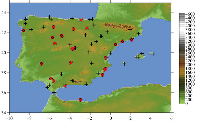
Figure 1. The Iberian Peninsula with its orography detailed with the mean wind speed stations in red crosses and the wind gust stations in black crosses.
3. Extreme Wind Speeds-Large Scale Atmospheric Patterns Connections
3.1. Large-Scale Atmospheric Patterns—Wind Speed Statistical Mode Relationships
A Principal Component Analysis (PCA) is applied to the MWS and Z1000 fields in order to know its general behaviour and to extract the most significant patterns from the original data [36]. However beyond mere data compression, a PCA is a very useful tool for exploring large multivariate data sets because of its potential for yielding substantial insights into both the spatial and temporal variations of the analysed fields. This methodology applied to spatial data enables patterns to be identified that can be attributed to specific physical processes by statistical assessment. The new uncorrelated variables are called principal components (PCs) and consist of linear combinations of the original variables derived from the diagonalization of the covariance/correlation matrix. The coefficients of the linear combinations represent the weight of the original variables in the PCs and they are named loadings or PC patterns. The PCs indicate modes of variation of the original field and are numbered according with their related variance. Thus, the first PC is the linear combination with the maximum possible variance; the second one is the linear combination with the maximum possible variance which is uncorrelated with the first PC and so on. The projection of the original series onto each eigenvector gives as result the time-dependence coefficient named scores or PC time series. In our case, the PCA was applied to the correlation matrices of both data sets, the MWS and Z1000 fields, being a set of eigenvalues and eigenvectors produced for each data set. Generally, the most important (the first ones) eigenvectors tend to describe regions with largest fluctuations. Thus, most relevant information from the data can be represented using fewer numbers of the principal components and a much smaller data set. Five leading modes for both datasets have been selected (not all shown). They account for more than 66% and 77% of the total variability for MWS and Z1000, respectively.
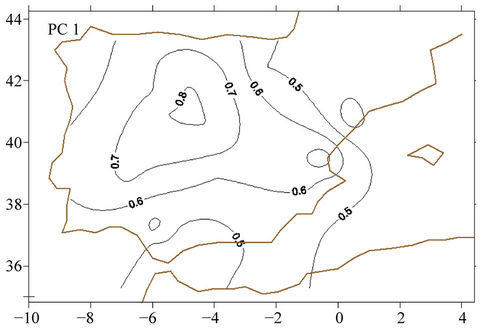
For reasons of brevity only the first mode is shown. In Figure 2(a), the eigenvector or spatial pattern of the retained MWS PCs is shown which helps highlighting diverse areas of different wind behaviour over Spain. The leading wind PC pattern (Figure 2(a)) accounts for the most important percentage of variance in the original data (37.9%). In Figure 2(a) the spatial pattern shows homogeneous wind behaviour in inner Iberia, and also underlines the area to the North Iberian Plateau with high correlation values. This conduct in the wind field could be related to the predominant westerly circulation regime (Poniente) in the Iberian Peninsula. The time variability of the spatial pattern above described is depicted showing the evolution of its PC time series obtained by applying the PCA over the MWS data in wintertime (Figure 2(b)). Significant trends are not found after applying a Mann-Kendall test and a spectral analysis of the PC time series. As stated previously, the first spatial pattern of Figure 2a showed homogeneous wind pattern over Iberia, underlying areas corresponding to the North Iberian Plateau. This behaviour can also be represented in the corresponding time series (Figure 2(b)) with mostly positive and high score values over the selected period (1970-2002).
However, the derived modes are statistically obtained. To analyze the extreme situations is needed to find connections between wind speed and the atmospheric field.
 (a)
(a)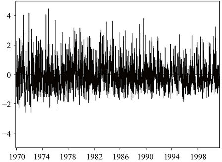 (b)
(b)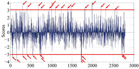 (c)
(c)
Figure 2. (a) Spatial patterns of the first PC of wind speed. The positive (negative) correlations are solid (dashed); (b) Time series of the first PC of the wind speed. Units are in standard deviations in the y-axis and the x-axis corresponds to the time period; (c) Illustration of picked up dates from the PC time series. Red rows indicate both the 5% high positive and negative scores used to build the composite maps.
Thus, to examine the real atmospheric circulation features associated with the winter wind speed patterns a set of positive and negative composite plots (of Z1000 and MWS) was constructed from the dates associated with 5 and 95 percentiles of the scores of the time series obtained of the PCA (Figure 2(c)). The composite maps represent configurations of the variable which are comparable to observations. Composites are defined here as the averaged ensemble of sets of maps of the large-scale atmospheric variable and the wind speeds [37]. Physical distinctive features in the composite plots are achieved through obtaining additional information to the statistical meaning of the derived spatial modes. Here, the anomaly composites of large-scale atmospheric variables have been built for those weather configurations associated with the highest and lowest PC scores of the wind speed. This way, the composites represent the atmospheric state associated with particular extreme wind characteristics. Positive (negative) composites are constructed directly from a number of configurations with high (low) scores of the PC time series because they indicate situations in which the corresponding PC mode is dominant in its positive (negative) phase. The selected number of configurations represents 5% of the total number of cases in the dataset.
Figure 3 shows the anomaly composites for Z1000 displaying the positive and negative composite plots conditioned by the 5% highest and lowest PC scores of the MWS. Subsequently, mean maps of Z1000 anomalies are drawn up from these days, and highlight the mean atmospheric state conditioned by predominant oscillation of the selected wind speed PC mode. Additionally, maps of MWS, also corresponding to those days, are picked up to illustrate the behaviour of the wind speed field over Spain in such atmospheric situations. Thus, the Z1000 anomaly composites associated to the first wind speed PC (Figures 3(a) and (b) first positive and negative composites) highlight two different mean atmospheric situations associated with the wind behaviour. Thus, in the first positive anomaly composite (Figure 3(a)), a strong gradient of Z1000 is observed over the Iberian Peninsula, underlying strong winds over Iberia as it can be noted in Figure 3(c) with wind speeds exceeding 8 m∙s−1 (30 km∙h−1) in daily average. In contrast to this atmospheric situation, the first negative composite (Figure 3(b)) displays high anomaly pressure over Iberia with little gradient over it and a nucleus over northern France. This situation is indicative of low wind speed
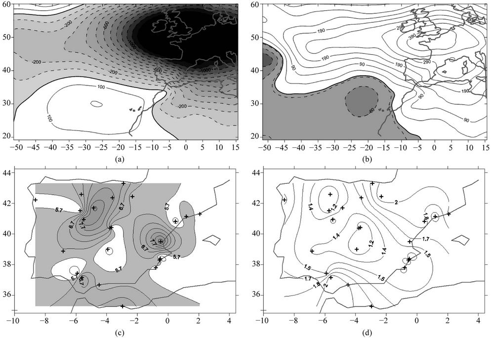
Figure 3. Composite maps of the Z1000 (gpm) conditioned by the highest and lowest scores of the first wind speed PC: (a) positive composite; (b) negative composite. Composite maps of wind (m∙s−1): (c) positive composite and (d) negative composite with shaded areas highlighting mean wind speed higher than 5 m∙s−1. Crosses indicate the wind stations.
over most of the area (Figure 3(d)).
3.2. Wind Speed Cumulated Probability— Large-Scale Atmospheric Statistical Mode Relationships
The relationships between MWS and large-scale atmospheric circulation are studied by means of wind speed cumulated probabilities associated with statistical modes of Z1000. To do this, the interactions between the PCs of Z1000 (only shown some results) and the observational local MWS are provided and analyzed. Thus, plots with cumulated probability values of wind speed associated with the highest and lowest scores of the Z1000 PC (not all shown) are described. These plots provide a fair idea about the observational wind frequency distributions conditioned by the different strong scores of the PC Z1000 time series.
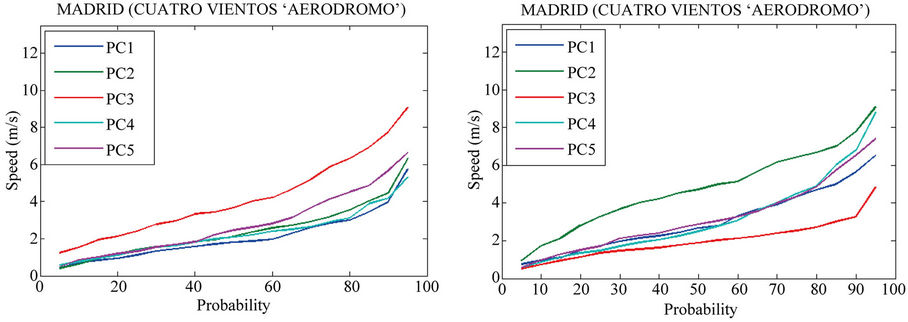
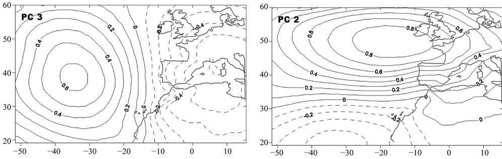
In order to have an idea about the wind speed cumulated frequencies these are derived associated to dominant positive and negative scores of the Z1000 PCs. To do this, higher and lower Z1000 scores were selected and subsequently their associated dates. Thus, at every stationthe MWS is picked up for such days and depicted the associated cumulative probabilities from 0 to 100%. Here only the Madrid station results are shown (Figures 4(a) and (b)). Once the PCA has been applied to the Z1000 field, the five leading Z1000 PCs, explaining 77% of the total variability, are retained. In general, it is remarkable in Figure 4(a) the quite high mean wind speeds associated with the Z1000 PC3. The third most significant PC pattern obtained for the Z1000 field (Figure 5(a)) consists of a configuration of positive (negative) correlation values centered over the North Atlantic area (western Mediterranean). This distribution of isolines implies that northern (southern, in its negative phase) winds are mainly affecting Iberia. Such configuration is associated with dynamically coherent and characterized by intrusions of cold (warm, in its negative phase) air masses over Iberia. This third Z1000 mode has the strongest influence over the observational wind speeds in throughout Spain, with daily MWS of up to 10 m∙s−1 in Madrid station (Figure 4(a)) and of almost 14 m∙s−1 (50 km∙h−1) in Melilla and Valencia (not shown) which reflects strong winds over such areas.
Figures 4(c)-(d) display the results of the cumulative
 (a)
(a)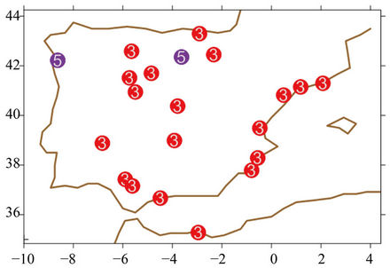 (b)
(b)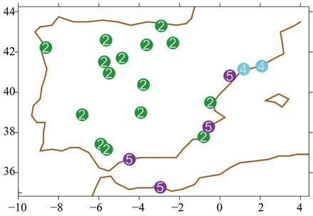 (c)
(c)
Figure 4. Wind speed cumulated frequencies associated with the strong (a) positive and (b) negative scores of the Z1000 principal components for the Madrid station. Dominant PCs (in numbers) over stations obtained from the higher area values of the wind speed cumulated frequency curves for (c) positive and (d) negative PC scores.
probabilities (in terms of the curve area values) for all used stations over Iberia. These maps show the leading PC in the wind speed pattern. Thus, for the high positive scores of the Z1000, higher values of the probability curve areas correspond to the third PC (Figure 4(c)). As noted above, this dominant mode showed a configuration characterized by intrusions of cold (warm, in its negative phase) air masses over Iberia. On the contrary, Figure 4(d) shows the results of the dominant PCs associated with the largest area under the probability curves derived from the strong negative scores of the PCs. As a result, the second PC of Z1000 (Figure 5(b)) is the leading mode for the negative PC scores (see also Figure 4(b)). Such PC make it possible to underline the fact that when high positive correlation values are located over western Britain Isles and the negative ones do it over southern Atlantic Ocean, the “Spanish” wind speed principally tends to deploy a homogeneous arrangement except for some stations in the eastern Iberian Peninsula. It can be noted the nearly dominance of the PC5 in most of the Spanish Mediterranean coast stations. This PC5 (Figure 5(c)) presents, in its positive phase, a spatial pattern similar to the second mode except for the center of negative anomalies which is located in between two strong nuclei of positive ones. The isolines are longitudinally extended which embodies strong southern (northern, in its negative phase) air advection over Iberia. In its negative phase, this situation resembles an omega blocking situation [38]. This persistent and particular configuration reflects a blocking pattern named “Omega block” with a meridionally-oriented high sandwiched in between two lows. At upper level, this kind of configuration can usually be characterized by a stationary ridge standing to the east of the Atlantic Ocean and by a main trough situated over the western Mediterranean zone which promotes longitudinal incursions of maritime cold air which comes from high latitudes and flows into the Western Mediterranean area after rotating around a cut-off low nearby the Iberian Peninsula. In the region of the blocking, the weather remains essentially unchanged, as any transient weather disturbances are forced to circumvent the block. Once established, major blocking situations tend to persist for at least a week and appear to represent some quasi-equilibrium state of the atmosphere. Therefore, the PC5 configuration presents an isoline-correlation gradient and shows changes in the isoline signs. Such
 (a)
(a)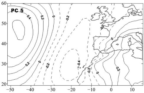 (b)
(b)
Figure 5. Spatial patterns of the obtained modes corresponding to Z1000: (a) third PC; (b) second PC and (c) fifth PC. The positive (negative) correlations are solid (dashed).
situation promotes advection of southern (northern) air masses over the Spanish Mediterranean coast.
4. Extreme Wind Speed and Wind Gust Estimations
In this section some techniques for estimating and forecasting wind speeds will be reviewed, with special emphasis in extreme winds. The improvement of meteorological forecasts of wind has been progressing by means of dynamic limited area modeling or by ensemble prediction systems, among other methodologies [39,40]. However, these methodologies bear high computational costs. In order to overcome this problem, the constructed analogue method in a framework of temporal prediction can be used [25,41].
The ANPAF downscaling analog model is used to obtain daily MWS and daily WGU over Spain [42]. The idea is based on the comparison between the field of an input variable and the other input variable to determine the greatest similarity between them. Here the Z1000 data are used both as input or historical reference field with which to be compared. Because of the great amount in the freedom degrees of any large-scale atmospheric field it turns out to be necessary to use long datasets, meaning a disadvantage of the methodology. However, if a high number of freedom degrees are considered as associated noise, then the inherent noise in the data can be reduced by a previous smoothing process. Thus, a PCA is previously applied to the Z1000 data base, the obtained PCs being the historical reference field. On the other hand, several distances based on Euclidean distance functions, have been defined and validated. The search of analogue patterns is based on finding a time that minimizes such distances in the PCA space.
Following this procedure, the methodology based on analogies has been applied to the Z1000 field in order to find several analogues to a particular Z1000 input pattern taking into account the above described distances. The ANPAF method used here can be mainly illustrated in the diagram of Figure 6. In the Figure 6, an input field score of the Z1000 corresponding to a day to be analogued,  , is compared with the different scores (stk and
 ) of the several obtained PCs of the Z1000 field by using the distance functions (dt and
 ) in order to find the most similar scores throughout the historic scores time record.

Figure 6. Illustration of the ANPAF analog method.
The procedure is crossvalidated by finding different analogues for a Z1000 input day and repeating the process for all the historic time record. Finally, a set of Z1000 analogues is obtained with the distance  (Pascual et al., 2012). Once the closest scores have been obtained throughout the time, their corresponding concomitant dates present associated wind and gust data that finally allow us that an estimated winds and gust can be obtained. The estimation can be made by using different criterions: a single analogue, average analogues, neural networks, …[29,43,44]. Here, the mean winds and gust obtained from the analog method have been estimated by using arithmetical means of several analogues. The tests cases have been analyzed by taking into account both deterministic and probabilistic tools to assess the accuracy and skill of the wind estimations.
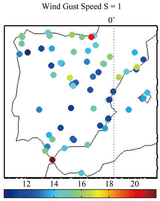
From the ANPAF model similar atmospheric situations were isolated and from them, a number of different wind fields (MWS and MGU) subsequently obtained and averaged to characterize and provide both estimated Spanish wind fields. In order to assess the accuracy and skill of the wind estimations these fields have been analyzed by means of both deterministic and probabilistic tools. Deterministic results point to a reasonable method skillful in estimating the MWS and the WGU fields in Spain. Concerning some probabilistic tools, rank histograms, reliability curves and skill scores have been used assessing the model skill in estimating wind data. In order to give an idea about the WGU values in Spain, Figure 7 displays the WGU values computed taking into account several thresholds corresponding with the values of the standard deviation, σ, of the original data. For values exceeding 2σ, all stations showed higher wind speeds than 58 km∙h−1, which corresponds to strong winds, reaching some stations values greater than 80 km∙h−1 that correspond to very strong winds.
Deterministic results are calculated for both wind vari-
 (a)
(a)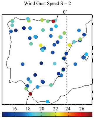 (b)
(b)
Figure 7. WGU values (m∙s−1) for different thresholds: (a) σ = 1, (b) σ = 2.
ables (Table 1). Biases for MWS and WGU between the averaged wind obtained from the analog method and the observational wind fields present small values. Moreover, the absolute relative biases present values around 1.66% and 1.81% for WGU and MWS, respectively, indicating that the estimated analog wind reproduces pretty well the observed winds. The values point to significant relationships in which the input and the output data are strongly related. Therefore, the input in the model (Z1000) involves enough information in the output (Z1000) fields, and consequently in the wind. Although the rmse values are in general small, the results of MWS and WGU are not comparable between them because of the different range of variability of each variable. On the other hand, the moderately high values of correlation highlight the relationships between the input and the output fields, thereby emphasizing a degree of skill of the method in estimating the MWS and the WGU at Spain.
From the deterministic point of view, different statistical tools have been used to compare the results of the MWS and the WGU. On the other hand, the probabilistic performance of wind estimations can be evaluated following the difference between a forecast probability distribution and the observed probability distribution. Thus, several probabilistic verification results are also shown in addition to the deterministic verification: rank histograms, reliability curves and skill scores have been used assessing the model skill in estimating wind data.
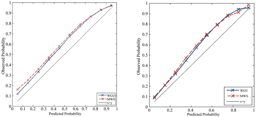
For the MWS rank histogram (not shown) large spread has been observed, which allows to highlight the presence of several observations located between the extremes of the analog estimations. The MWS Talagrand also presents an asymmetric shape, pointing out some underprediction of the MWS values. The WGU rank histogram has shown flatter distribution than the MSW one, illustrating a general pretty better behaviour. The reliability curves have been computed taking into account several thresholds corresponding with the values of the standard deviation, σ, of the original data, both MWS and WGU. For all the thresholds (Figure 8) the reliability curves deviate in general from the best line, the model forecast probability being smaller than observed frequency. This situation indicates an underestimation of the observational wind frequencies in both variables.
Again, the WGU performance is quite better than the MWS one. It is worth noting the resemblance of the un-
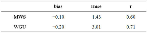
Table 1. Spatial averaged bias (m∙s−1), rmse (m∙s−1) and correlation obtained from the estimated wind versus the observational data.
derestimation of the probabilistic values in all reliability diagrams for all thresholds. It points out that the ANPAF model reasonably matches the observational and forecast data.
Additionally, and in accordance with Brier [45], the Brier Score (BS) and the Brier Skill Score (BSS) are here used and derived with respect to the climatological probability for different thresholds. The BS shows that the goodness of the model performance as measured by this score is very similar to the different thresholds. The BSS proves that the model generates forecasts with better skill than the climatology. The lower the Brier Score the better forecast; so, as much as the BSS tends to the unity, better is the model skill. The BSS is typically defined as the relative probability score compared with the probability score of a reference forecast. In order to assess the accuracy and skill of all obtained wind estimations from the analogue model, the BSS has been also derived herein for values of the standard deviation of the original data, both MWS and WGU. Thus, not only the model mean skill is analyzed, but the estimated tails are also evaluated. The BS of reference, BSref, used herein corresponds to the climatological value. The BSref has been obtained using the observational climatological frequencies taking into account such thresholds. The areal averaged BSSs for all selected thresholds show values greater than zero and indicate that the forecasts improve the model. The BSSs for several σs show an asymmetric shape (Figure 9), the best results being associated with the value of σ = 0.5 in both cases, although the WGU result is better than the MWS one. The analogs obtained from the ANPAF model shows the best results for σ values ranging between 0.5 and 1.5. For extreme values, associated with the BSS ≈ 0.12 for σ ≥ 2, a gust range of 16 - 26 m∙s−1 is recorded, with very strong winds spreading over the Ebro Valley and the Gibraltar Strait (≈93 km∙h−1). It is worth noting that MWS and WGU extreme values show similar behaviour.
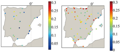
The BSSs for MWS and WGU are also derived for mean values (Figure 10) and for σ = 0.5 (not shown) in each Spanish station. The BSS spatial distribution is shown more clearly in the WGU case than in the MWS one for both thresholds, since the WGU database includes more stations than the MWS dataset. The MWS BSS results (Figure 10(a)) are again worse than the corresponding WGU ones (Figure 10(b)) in the whole domain. For both thresholds, the BSS spatial distribution presents the best values (≈0.25) over Northern Iberia (Figure 10(b)), while the rest of stations show small values. It means that the atmospheric situations coming from the Atlantic Ocean are better to predict mean wind and gusts in the Northern Peninsula. It is worth also to note high WGU BSS values located over the Gibraltar Strait and along the Ebro Valley zones, although smaller
 (a)
(a) (b)
(b)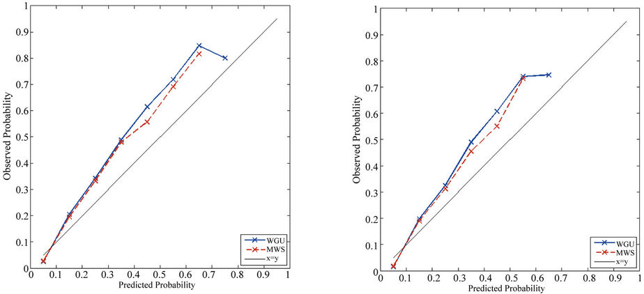 (c)
(c)
Figure 8. Reliability diagrams of MWS (red dashed line) and WGU (blue continuous line) derived for different thresholds: (a) σ = 0; (b) σ = 0.5; (c) σ = 1.0; (d) σ = 1.5; (e) σ = 2.0 and (f) σ = 2.5.
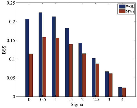
Figure 9. Illustration of BSS values for different values of σ: red bars (MWS) and blue bars (WGU).
 (a) (b)
Figure 10. Spatial distributions of BSS for σ = 0 of: (a) MWS and (b) WGU stations shown in Figure 1.
ones in the MWS case. On the contrary, poorer BSS estimations and thereby poorer prognosis are expected to be mainly located on northern Catalonia for both σ = 0.5 values and for the mean values.
5. Conclusions
The relationships between observed wind speeds in Spain and surface circulation patterns have been examined with special emphasis in extreme winds. The analysis, based on composite maps built from extreme data of PC modes of the large-scale atmospheric field, has shown different mean atmospheric situations associated with wind patterns and with strong gradients of Z1000 are related to moderate to strong wind in Spain. The analyses have revealed a strong influence of the pressure centers over the Atlantic Ocean in the Spanish wind speed field and also allowed to identify a number of atmospheric circulation patterns that govern the wind speed variability at Spain. The PCA and the associated analyses based on composites and wind speed cumulated probabilities together with their under curve area values have shown that the atmospheric dynamics in the North Atlantic is responsible for much of the Spanish wind speed variability. The variation of intensity and/or position of pressure centers, within a climate change scenario, could possibly change the relative frequency of the large-scale atmospheric patterns or form new ones, changing the present wind regime.
Additionally, it has been revised the process to estimate wind fields based on finding analogs. The ANPAF model is used to find similar atmospheric patterns, and from them to obtain wind fields. In order to assess the accuracy and skill of the wind estimations these fields have been analyzed by means of both deterministic and probabilistic tools. The significantly close relationships between the input and the output data, and hence with the wind are shown by bias and correlation estimators. Reliability curves indicate some underestimation in the model results of the observational wind frequencies in both variables. The WGU behaviour is quite better than the MWS one, in general. It is worth noting the resemblance of the underestimation of the probabilistic values in all reliability diagrams for all thresholds except for the small probabilistic values for σ ≥ 1 (gusts greater than 80 km∙h−1, which corresponds to very strong winds). For extreme wind values MWS and WGU show similar behaviour, and gusts of up to 26 m∙s−1 are recorded corresponding to BSS ≈ 0.12 for σ ≥ 2. On the other hand, the BSS spatial distribution presents the best values (≈0.25) over the northern area, emphasizing that the atmospheric situations coming from the Atlantic Ocean are better to predict mean wind and gusts in the Northern Peninsula. It may be concluded that the process to find analogs and the subsequent application of the ANPAF analog model can be considered as a good technique to find similar atmospheric patterns, and from them to estimate wind fields.
6. Acknowledgements
This work has been partially supported by the research projects CGL2011-25327, UE Safewind G.A. No. 21374, VA025A10-2 and AYA2011-29967-C05-02. The authors wish to thank the Spanish Meteorological Agency (AEMET: Agencia Estatal de Meteorología) for providing the Spanish wind datasets and the European Centre for Weather Medium Forecast (ECWMF) for providing the ERA40 data.
REFERENCES
- “Swiss Re,” 2000. http://www.swissre.com/about_us/art_architecture/Swiss_Re_Next.html
- U. Ulbrich, A. H. Fink, M. Klawa and J. G. Pinto, “Three extreme storms over Europe in December,” Weather, Vol. 56, No. 3, 2001, 1999, pp. 70-80. doi:10.1002/j.1477-8696.2001.tb06540.x
- J. I. Barredo, “No Upward Trend in Normalised Windstorm Losses in Europe: 1970-2008,” Natural Hazards of Earth System Sciences, Vol. 10, 2010, pp. 97-104. doi:10.5194/nhess-10-97-2010
- J. P. Palutikof, P. M. Kelly, T. D. Davies and J. A. Halliday, “Impacts of Spatial and Temporal Windspeed Variability on Wind Energy Output,” Journal of Applied Meteorology, Vol. 26, No. 9, 1987, pp. 1124-1133. doi:10.1175/1520-0450(1987)026<1124:IOSATW>2.0.CO;2
- R. H. Thuilleier, “Real-Time of Local Wind Patterns for Application to Nuclear-Emergency Response,” Bulletin of the American Meteorological Society, Vol. 68, No. 9, 1987, pp. 1111-1115. doi:10.1175/1520-0477(1987)068<1111:RTAOLW>2.0.CO;2
- J. A. Zuranski and B. Jaspinka, “Directional Analysis of Extreme Wind Speeds in Poland,” Journal of Wind Engineering and Industrial Aerodynamics, Vol. 65, No. 1-3, 1996, pp. 13-20. doi:10.1016/S0167-6105(97)00018-4
- M. Gaya, J. Amaro, M. Aran and M. C. Llasat, “Preliminary Results of the Societal Impact Research Group of MEDEX: The Request Database (2000-2002) of Two Meteorological Services,” Proceedings of 9th EGS Plinius Conference, Nisosia, 2008, p. 12.
- J. Amaro, M. Aran, L. Barberia and M. C. Llasat, “The Strong Wind Event of 24th January 2009 in Catalonia: A Social Impact Analysis,” Proceedings of 10th EGS Plinius Conference, Barcelona, 2009, p. 10.
- M. J. OrtizBeviá, E. SánchezGómez and F. J. AlvarezGarcía, “North Atlantic Atmospheric Regimes and Winter Extremes,” Natural Hazards and Earth System Science, Vol. 11, 2011, pp. 971-980. doi:10.5194/nhess-11-971-2011
- J. Tastu, P. Pinson, E. Kotwa, H. Aa. Nielsen and H. Madsen, “Spatio-Temporal Analysis and Modeling of Wind Power Forecast Errors,” Wind Energy, Vol. 14, No. 1, 2011, pp. 43-60. doi:10.1002/we.401
- P. Pinson, G. Papaefthymiou, B. Klockl, H. Aa. Nielsen and H. Madsen, “From Probabilistic Forecasts to Statistical Scenarios of Short-Term Wind Power Production,” Wind Energy, Vol. 12, No. 1, 2009, pp. 51-62. doi:10.1002/we.284
- P. Pinson and H. Madsen, “Adaptive Modeling and Forecasting of Wind Power Fluctuations with MarkovSwitching Autoregressive Models,” Journal of Forecasting, Vol. 31, No. 4, 2012, pp. 281-313. doi:10.1002/for.1194
- P. Pinson, H. Aa. Nielsen, H. Madsen and G. Kariniotakis, “Skill Forecasting from Ensemble Predictions of Wind Power,” Applied Energy, Vol. 86, No. 7-8, 2009, pp. 1326- 1334. doi:10.1016/j.apenergy.2008.10.009
- M. L. Martín, D. Santos-Muñoz, F. Valero and A. Morata, “Evaluation of an Ensemble Precipitation Prediction System over the Western Mediterranean Area,” Atmospheric Research, Vol. 98, No. 1, 2010, pp. 163-175. doi:10.1016/j.atmosres.2010.07.002
- M. Y. Luna, M. L. Martín, F. Valero and F. GonzálezRouco, “Wintertime Iberian Peninsula Precipitation Variability and Its Relation to North Atlantic Atmospheric Circulation,” In: M. Brunet and D. López, Eds., Detecting and Modelling Regional Climate Change and Associated Impacts, Springer-Verlag, Berlin, 2001, pp. 369-376. doi:10.1007/978-3-662-04313-4_31
- F. Valero, M. Y. Luna, M. L. Martín, A. Morata and F. González-Rouco, “Coupled Modes of Large-Scale Climatic Variables and Regional Precipitation in the Western Mediterranean in Autumn,” Climate Dynamics, Vol. 22, No. 2-3, 2004, pp. 307-323. doi:10.1007/s00382-003-0382-9
- M. L. Martín, M. Y. Luna, A. Morata and F. Valero, “North Atlantic Teleconnection Patterns of Low-Frequency Variability and Their Links with Springtime Precipitation in the Western Mediterranean,” International Journal of Climatology, Vol. 24, No. 2, 2004, pp. 213-230. doi:10.1002/joc.993
- M. L. Martín, F. Valero, A. Morata, M. Y. Luna, A. Pascual and D. Santos-Muñoz, “Springtime Coupled Modes of Regional Wind in the Iberian Peninsula and LargeScale Variability Patterns,” International Journal of Climatology, Vol. 31, No. 6, 2011, pp. 880-895. doi:10.1002/joc.2127
- M. L. Martín, F. Valero, A. Pascual, A. Morata and M. Y. Luna, “Springtime Connections between the Large-Scale Sea Level Pressure Field and Gust Wind Speed over Iberia,” Natural Hazards of Earth System Sciences, Vol. 11, 2011, pp. 191-203. doi:10.5194/nhess-11-191-2011
- E. García-Ortega, L. López and J. L. Sánchez, “Atmospheric Patterns Associated with Hailstorm Days in the Ebro Valley, Spain,” Atmospheric Research, Vol. 100, No. 4, 2011, pp. 401-427. doi:10.1016/j.atmosres.2010.08.023
- R. Frouin, A. F. Fiúza, I. Ambar and T. J. Boyd, “Observations of a Poleward Surface Current off the Coasts of Portugal and Spain during the Winter,” Journal of Geophysical Research, Vol. 95, No. C1, 1990, pp. 679-691. doi:10.1029/JC095iC01p00679
- R. D. Haynes and E. D. Barton, “A Poleward Flow along the Atlantic Coast of the Iberian Peninsula,” Journal of Geophysical Research, Vol. 95, No. 1, 1990, pp. 11425- 11442. doi:10.1029/JC095iC07p11425
- P. Bougeault, B. Benech, P. Bessemoulin, B. Carissimo, A. Lar, J. Pelon, M. Petitdidier and E. Richard, “PYREX: A Summary of findings,” Bulleting American Meteorological Society, Vol. 78, No. 4, 1997, pp. 637-650. doi:10.1175/1520-0477(1997)078<0637:PASOF>2.0.CO;2
- F. Valero, Y. Luna and M. L. Martín, “An Overview of a Heavy Rain Event at Southeastern Iberia: The Role of the Large-Scale Meteorological Conditions,” Annales Geophysicae, Vol. 15, 1997, pp. 494-502. doi:10.1007/s00585-997-0494-3
- E. N. Lorenz, “Atmospheric Predictability as Revealed by Naturally Accourring Analogues,” Journal of Atmospheric Science, Vol. 26, No. 4, 1969, pp. 636-646. doi:10.1175/1520-0469(1969)26<636:APARBN>2.0.CO;2
- T. Hastie, R. Tibshirani and J. Friedman, “The Elements of Statistical Learning,” Springer, New York, 2001. doi:10.1007/978-0-387-21606-5
- J. Fernandez and J. Saenz, “Improved Field Reconstruction with the Analog Method: Searching the CCA Space,” Climate Research, Vol. 24, No. 3, 2003, pp. 199-213. doi:10.3354/cr024199
- K. Fraedrich, C. C. Raible and F. Sielmann, “Analog Ensemble Forecasting of Tropical Cyclone Tracks in the Australian Region,” Weather and Forecasting, Vol. 18, 2003, pp. 3-11.
- E. Y. Zorita and H. von Storch, “The Analog Method as a Simple Statistical Downscaling Technique: Comparison with More Complicated Methods,” Journal of Climate, Vol. 12, No. 8, 1999, pp. 2474-2489. doi:10.1175/1520-0442(1999)012<2474:TAMAAS>2.0.CO;2
- R. L. Wilby and T. Wigley, “Downscalling General Circulation Model Output. A Review of Methods and Limitations,” Progress in Physical Geography, Vol. 21, No. 4, 1997, pp. 530-548. doi:10.1177/030913339702100403
- H. M. Dool van den, “Searching for Analogs, How Long Must We Wait?” Tellus, Vol. 46A, 1994, pp. 314-324.
- A. Pascual, M. L. Martin, F. Valero, D. Santos-Muñoz,, A. Morata and M. Y. Luna, “Development of an Analogous Model for Wind Prediction Using Principal Components,” The SAFEWIND Workshop, Oldemburg, 2010, 22 p. www.safewind.eu
- A. Morata, M. L. Martín, M. G. Sotillo, F. Valero and M. Y. Luna, “Iberian Autumn Precipitation Characterization through Observed, Simulated and Reanalysed Data,” Advances of Geosciences, Vol. 16, 2008, pp. 49-54. doi:10.5194/adgeo-16-49-2008
- F. Valero, M. L. Martín, M. G. Sotillo, A. Morata and M. Y. Luna, “Characterization of the Autumn Iberian Precipitation from Long-Term Data Sets: Comparison between Observed and Hindcasted Data,” International Journal of Climatology, Vol. 29, No. 4, 2009, pp. 527- 541. doi:10.1002/joc.1726
- A. J. Simmons and J. K. Gibson, “The ERA-40 Project Plan,” ERA-40 Project Report Series No. 1. ECMWF, Reading, 2000.
- R. W. Preisendorfer, “Principal Component Analysis in Meteorology and Oceanography,” Elsevier Science Publishers BV, Amsterdam, 1998.
- A. Pascual, M. L. Martín, F. Valero, M. Y. Luna and A. Morata, “Wintertime Connections between Extreme Wind Patterns in Spain and Large-Scale Geopotential Heath Field,” Atmospheric Research, Vol. 122, 2013, pp. 213- 228. doi:10.1016/j.atmosres.2012.10.033
- H. B. Bluestein, “Synoptic Dynamic Meteorology in Midlatitudes. Vol. II. Observations and Theory of Weather Systems,” Oxford University Press, Oxford, 1993.
- T. M. Hamill, “Interpretation of Rank Histograms for Verifying Ensemble Forecasts,” Monthly Weather Review, Vol. 129, 2001, pp. 550-560. doi:10.1175/1520-0493(2001)129<0550:IORHFV>2.0.CO;2
- P. Pinson and R. Hagedorn, “Verification of the ECMWF Ensemble Forecasts of Wind Speed against Observations,” Meteorological Applications, Vol. 19, No. 4, 2012, pp. 484-500. doi:10.1002/met.283
- S. Herrera, S. Pazo, J. Fernández and M. A. Rodríguez, “The Role of Large-Scale Spatial Patterns in the Chaotic Amplification of Perturbations in a Lorenz’96 Model,” Tellus A, Vol. 63, No. 5, 2011, pp. 978-990. doi:10.1111/j.1600-0870.2011.00545.x
- A. Pascual, F. Valero, M. L. Martín, A. Morata and M. Y. Luna, “Probabilistic and Deterministic Results of the ANPAF Analog Model for Spanish Wind Field Estimations,” Atmospheric Research, Vol. 108, 2012, pp. 39-56. doi:10.1016/j.atmosres.2012.01.011
- A. S. Cofiño, “Técnicas Estadísticas y Neuronales de Agrupamiento Adaptativo Para la Predicción Probabilística de Fenómenos Meteorológicos Locales. Aplicación en el Corto Plazo y en la Predicción Estacional,” Tesis Doctoral, Universidad de Cantabria, Cantabria, 2004.
- J. M. Gutiérrez, R. Cano, A. S. Cofiño and M. A. Rodríguez, “Clustering Methods for Statistical Down-scaling in Short-Range Weather Forecast,” Monthly Weather Review, Vol. 132, No. 9, 2004, pp. 2169-2183. doi:10.1175/1520-0493(2004)132<2169:CMFSDI>2.0.CO;2
- G. W. Brier, “Verification of Forecasts Expressed in Terms of Probabilities,” Monthly Weather Review, Vol. 78, No. 1, 1950, pp. 1-3. doi:10.1175/1520-0493(1950)078<0001:VOFEIT>2.0.CO;2