American Journal of Climate Change
Vol.2 No.2(2013), Article ID:33529,10 pages DOI:10.4236/ajcc.2013.22011
Regional Climate Index for Floods and Droughts Using Canadian Climate Model (CGCM3.1)
1Department of Civil Engineering, Université de Moncton, Moncton, Canada
2Department of Fisheries and Oceans Canada, Moncton, Canada
Email: nassir.el-jabi@umoncton.ca
Copyright © 2013 Nassir El-Jabi et al. This is an open access article distributed under the Creative Commons Attribution License, which permits unrestricted use, distribution, and reproduction in any medium, provided the original work is properly cited.
Received November 23, 2012; revised December 28, 2012; accepted January 12, 2013
Keywords: Canadian Climate Model; Artificial Neural Networks; Floods; Droughts; Regional Climate Index
ABSTRACT
The impacts of climate change on the discharge regimes in New Brunswick (Canada) were analyzed, using artificial neural network models. Future climate data were extracted from the Canadian Coupled General Climate Model (CGCM3.1) under the greenhouse gas emission scenarios B1 and A2 defined by the Intergovernmental Panel on Climate Change (IPCC). The climate change fields (temperatures and precipitation) were downscaled using the delta change approach. Using the artificial neural network, future river discharge was predicted for selected hydrometric stations. Then, a frequency analysis was carried out using the Generalized Extreme Value (GEV) distribution function, where the parameters of the distribution were estimated using L-moments method. Depending on the scenario and the time slice used, the increase in low return floods was about 30% and about 15% for higher return floods. Low flows showed increases of about 10% for low return droughts and about 20% for higher return droughts. An important part of the design process using frequency analysis is the estimation of future change in floods or droughts under climate scenarios at a given site and for specific return periods. This was carried out through the development of Regional Climate Index (RCI), linking future floods and droughts to their frequencies under climate scenarios B1 and A2.
1. Introduction
There is currently a broad scientific consensus that the global climate is changing in ways that are likely to have a profound impact on human society and the natural environment over the coming decades. Climate change and its impacts on a global scale are the focus of intense, broad-based international research efforts in natural and social sciences. However, understanding the nature and potential consequences of climate change at regional scales remains a challenge. Moreover, it has been recognized that changes in the frequency and magnitude of extreme weather events are likely to have more substantial and widespread impacts on the environment and human activities than changes in the average climate.
A number of extreme events (with significant impacts on the environment and socio-economic activities) have been observed during the last decade, including severe floods and droughts as well as extreme heat around the world. These extreme events have caused serious risks to the health of populations as well as to ecosystems and have had severe economic consequences on sectors such as agriculture and water resources. Anticipating specific climatic impacts is thus, as much of a challenge in assessing risks and uncertainties than predicting future changes. As such, it is important: 1) to improve our ability to manage extreme climatic risks, 2) to assess the consequences of extreme events over the next decades, and 3) to develop new tools and design criteria to more accurately assess the impact of extreme events on water resources and river discharge (e.g., floods and droughts).
In Atlantic Canada over the next 100 years, the mean surface air temperature is expected to increase by 2 to 6˚C [1], contributing to potentially large reductions in streamflow [2,3] and significant impacts on aquatic resources [4]. The demand for water withdrawal from rivers (e.g. irrigation, drinking water, etc.) and maintaining adequate instream flow for the protection of aquatic resources are tenuously balanced, and represent an ongoing challenge in water resources management. Many rivers in eastern Canada have recently experienced record low flow conditions, coupled with record high water temperatures [5-7], and an increase in water withdrawal.
The study was carried out in New Brunswick, Canada (NB), which lies on Canada’s Atlantic coast. Rainfall, snowmelt, and groundwater all contribute to river flow, producing seasonal and annual variations. High flows are generally the result of spring snowmelt, although heavy rainfall can also cause high flows and floods, especially in small streams. Low flows generally occur in late summer, when precipitation is low and evaporation is high, and in late winter, when precipitation is stored until spring in the form of ice and snow.
Flood studies in New Brunswick, Canada (NB) were carried out over 20 years ago [8] and were recently updated [9], using two distributions functions, namely the 3-parameter lognormal (LN3) and the generalized extreme value (GEV) distributions.
In Aucoin et al. [9], single station analysis was carried out for the same hydrometric stations analyzed earlier by Environment Canada and New Brunswick Department of Municipal Affairs and Environment [8]. In addition, a regional flood frequency analysis was carried out using both regression equations and the index flood approach. In general, the results were consistent with those from early studies [8,9]. However, it was observed that updateing the flood information resulted, for many stations, in an improvement of flood estimates.
Low flows were also analysed in New Brunswick [10, 11]. This analysis consisted in fitting the Annual Minimum Flow (AMF) to a Type III extremal distribution (3- parameter Weibull) function and calculating the discharge for different recurrence intervals. The low flow frequencies were calculated for 1-day, 7-day and 14-day durations and for different recurrence intervals (e.g., 2-year, 10-year, 20-year and 50-year). Following the single station analysis, a regression analysis was carried out in order to estimate low flows on a regional basis and for ungauged basins. Missing from these previous studies were the projections of future floods and low flows conditions under climate change. As such, this aspect will be addressed within the present study.
2. Data and Method
The present study analyses the climate change impacts on the discharge regimes of several catchments in New Brunswick. The hydrological response for given climate scenarios was simulated using artificial neural network models. Future climate data were extracted from the Canadian Coupled General Climate Model (CGCM) under different greenhouse gas emission scenarios defined by the Intergovernmental Panel on Climate Change [12]. Using an artificial neural network model, future river discharge was predicted for selected hydrometric stations. A frequency analysis was then carried out using the above described distribution functions, and the parameters of the distribution were estimated using L-moments method [13].
2.1. Global Climate Model
General Circulation Models (GCMs) are based on mathematical representations of atmosphere, ocean, ice cap as well as land surface processes. These models are used for simulating the response of the global climate system to increasing “greenhouse gas” concentrations. Historically, gross CO2 emissions have increased at an average rate of 1.7% per year since 1900 [13] and if this trend continues, global emissions would increase more than six fold by 2100. Different scenarios have been presented by the Intergovernmental Panel on Climate Change (IPCC) [12] which reflects a variety of CO2 concentrations over the next 100 years. While the complexity of the global climate system is well captured by these models, they are unable to represent local scale features and processes due to their limited spatial resolution. Large geographic areas (e.g. 50,000 to 300,000 km2) represent the basic unit of GCMs. In the present study the Canadian Global Coupled Model CGCM 3.1/T63, from CCCma, (Canadian Centre for Climate Modeling and Analysis), was used. This model has a geographic areas represented by a grid of approximately 2.81˚ latitude by 2.81˚ longitude (~60,000 km2). In New Brunswick, a few grids points cover the entire province. At odds with GCM resolution is the fact that most researchers are focusing on the impacts of climate change primarily at the local and regional scales rather than focusing on large or global-scale changes. Therefore, downscaling of data is often used, and the delta change approach will also be used in the present study. The time-slice simulations follow the IPCC “observed 20th century” 20C3M scenario for years 1970-1999 and the Special Report on Emission Scenarios (SRES) B1 and A2 for years 2010-2100 [12].
2.2. Data Processing
Average temperatures in New Brunswick range from −10˚C in January to 19˚C in July. New Brunswick receives approximately 1100 mm of precipitation annually, with 20% to 33% falling in the form of snow [14]. Precipitation tends to be highest in southern parts of the province whereas the northern part of New Brunswick receives relatively higher amounts of precipitation in the form of snow due to colder winters.
Daily maximum and minimum air temperatures and total precipitation data from seven meteorological stations in New Brunswick were obtained from Environment Canada’s National Climate Data Archive (Table 1, Figure 1). Air temperature data were available from dates going back as far as 1895 for some stations whereas precipitation data goes back to 1929 (Aroostook). Daily
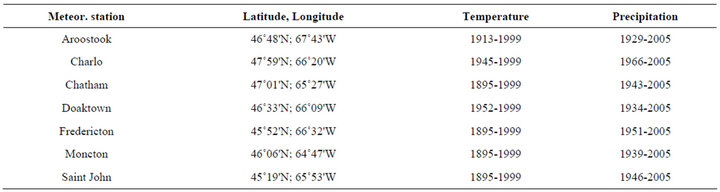
Table 1. Meteorological stations.
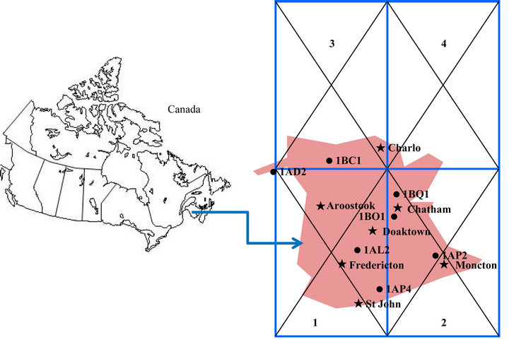
Figure 1. Subarea of 4 grid boxes corresponding to New Brunswick (box size ~200 × 300 km, • hydrometric station, × meteorological station).
discharge (m3/s) data from seven hydrometric stations in New Brunswick were obtained from Environment Canada’s National Water Data Archive (HYDAT CD-ROM) (Table 2, Figure 1). Basin size of analysed stations ranged between 668 km2 (Canaan River) and 14,700 km2 (Saint John River).
Simulated monthly maximum and minimum air temperatures and total precipitation for the period of 1970- 2100 was obtained from CCCma. The atmosphere model output was provided on a 128 × 64 Gaussian grid. Figure 1 shows the sub-region of four tiles corresponding to New Brunswick.
When using simulated data from the CCCma model, an Inverse Distance Weighting (IDW) method was used to compute data corresponding to each meteorological site. This is a method for multivariate interpolation, a process of assigning values to unknown points by using values from usually scattered set of known points. The interpolated data were then downscaled using delta change approach [15,16]. This approach to downscaling of GCMs for hydrological modeling is one of the simpler statistical downscaling techniques. In fact, Fowler et al. [17] noted that, if reproducing the mean characteristics are the main objectives, then simple statistical downscaling methods can perform as well as more sophisticated approaches. Changes in mean climate are applied as follows:
For air temperatures:
 (1)
(1)
For precipitation:
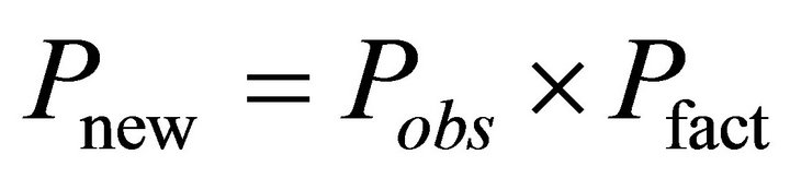 (2)
(2)
where ![]() is the difference between the GCM simulated mean temperature (from the future time period) and the historic mean temperature (1970-1999).
is the difference between the GCM simulated mean temperature (from the future time period) and the historic mean temperature (1970-1999).  is the ratio of the GCM simulated mean precipitation from the future time period relative to the historic period.
2.3. Hydrological Modelling Using Artificial Neural Networks
The average monthly discharge under climate change
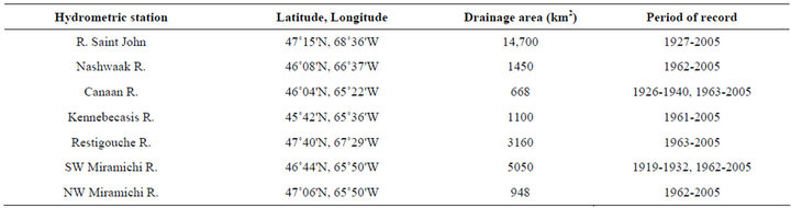
Table 2. Hydrometric stations.
was simulated first using the Artificial Neural Networks (ANN) and then extreme event characteristics (floods and low flows) were predicted using a regression model based on historical events (ratio of daily to monthly values). This was done for the period 1970 to 1999. ANN approaches have been successfully used in water resources in a wide variety of applications [18,19]. Applications in river flow and groundwater level forecasting as well as sediment estimation are a few examples. Also, predicting conductivity and acidity of streams are some of the time series successfully modeled using this technique [20].
The following ANN model was used to predict mean discharge,  .
.
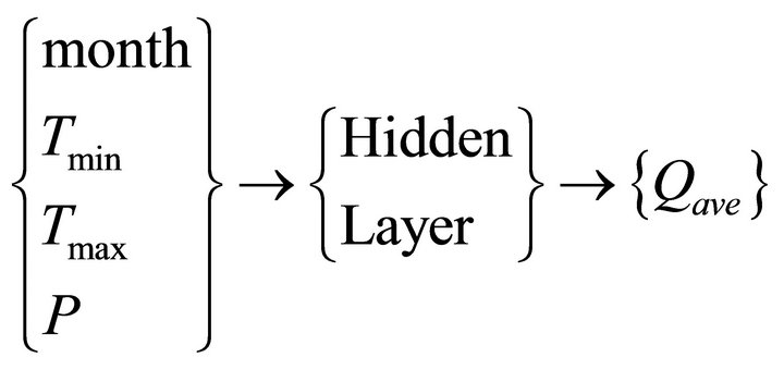
where month is the month of year (1, 2, ∙∙∙, 12), T is the air temperature (min or max) and P is the precipitation. The model is characterized by:
• Learning algorithm: back-propagation with Levenberg-Marquard method and early stopping;
• Training and validation data: 85% of data;
• Testing data: 15% of data;
• Hidden layer: 8 to 12 neurons.
It was observed that the extreme discharge events were better predicted using a 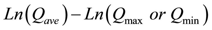 regression model. Therefore, average monthly discharge,
  , was simulated first using the ANN model. Once the
  was predicted, then the regression equations were used to link maximum (
 ) and minimum (
![]() ) daily flows during each month.
) daily flows during each month.
3. Results
3.1. Method Evaluation
The ANN model showed a coefficient of determination, R2, ranging between 0.69 and 0.79 in the prediction of monthly flows (1970-1999). High flow predictions showed higher R2 (0.85 - 0.92) than low flow predictions (0.66 - 0.82). Using the results from the Doaktown site (in close proximity SW Miramichi River) as an example, Figure 2 shows how well the ANN model coupled with a Ln-Ln model simulated monthly  ,
,  and
and ![]() between 1985 and 1990 compared to observed discharge values when using historical input data (precipitation and temperature). Results here are typical of the whole study period. This figure shows that simulated discharges coincided fairly well with the observed discharges. It should be noted that input data consisted of local historical observations at the Doaktown station. As such, the ANN model and regression equations were effective in predicting the different flow components using historical data [16].
between 1985 and 1990 compared to observed discharge values when using historical input data (precipitation and temperature). Results here are typical of the whole study period. This figure shows that simulated discharges coincided fairly well with the observed discharges. It should be noted that input data consisted of local historical observations at the Doaktown station. As such, the ANN model and regression equations were effective in predicting the different flow components using historical data [16].
3.2. Future Climate Change Projections
Tables 3-5, in annual means, summarize the major changes in temperatures, precipitation and average flows throughout the province of New Brunswick. In terms of mean air temperature, the current air temperature in New Brunswick is expected to increase by 1.2˚C (2010-2039), 2.2˚C (2040-2069) and 2.9˚C (2070-2099) under scenario B1 and 1.4˚C (2010-2039), 3.2˚C (2040-2069) and 5.2˚C (2070-2099) under scenario A2 (Table 3). Precipitation (mean annual precipitation) is projected to increase significantly compared to current climate conditions (Table 4). At Doaktown, the precipitation will most likely increase from approximately 1140 mm annually to 1200 mm annually (B1 scenario) and to 1440 mm annually (A2 scenario) within the next hundred years. This represents an increase in precipitation of 5.1% (B1) and 14.6% (A2) compared to current conditions. Greatest increases are projected at the Moncton site (Table 4). Other sites show similar increases depending on the time slice and climate scenario. In general, the mean annual precipitation is expected to increase by 2% - 6% under the B1 scenarios and by 5% - 15% under the A2 scenario for the province of New Brunswick.
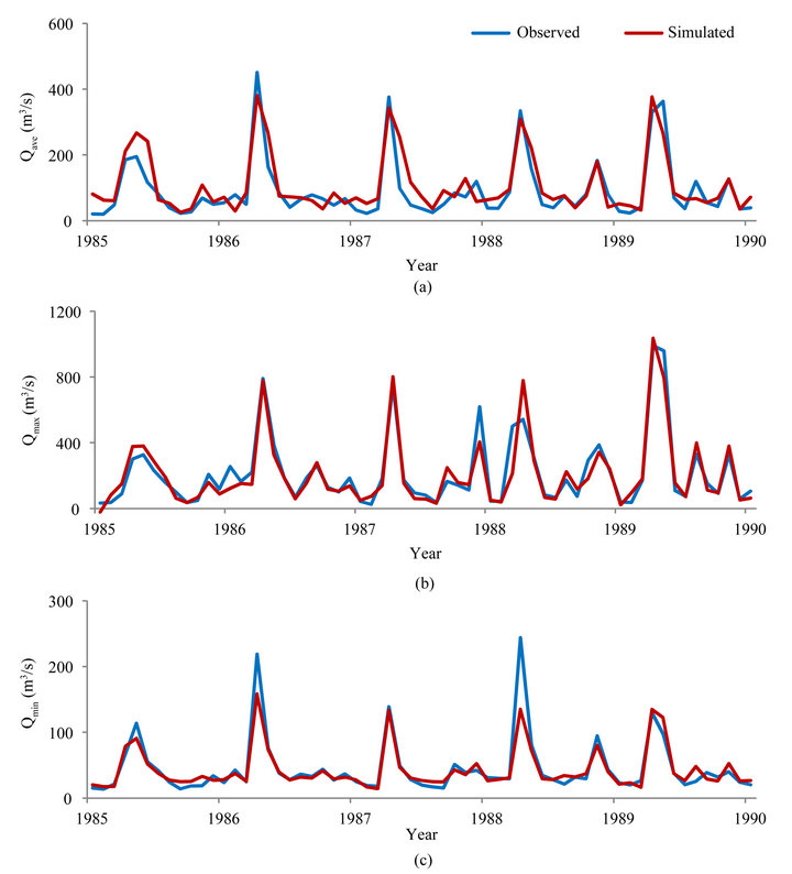
Figure 2. Observed and simulated monthly discharges for SW Miramichi River (a) mean discharge (b) maximum discharge (c) minimum discharge.
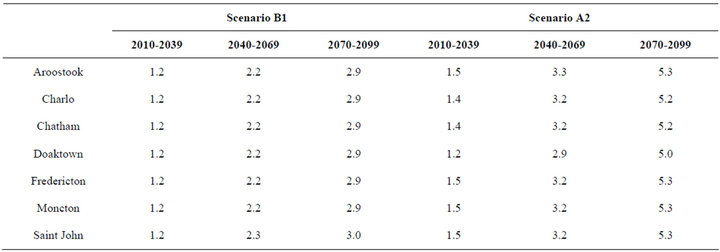
Table 3. Mean air temperature increase (˚C).
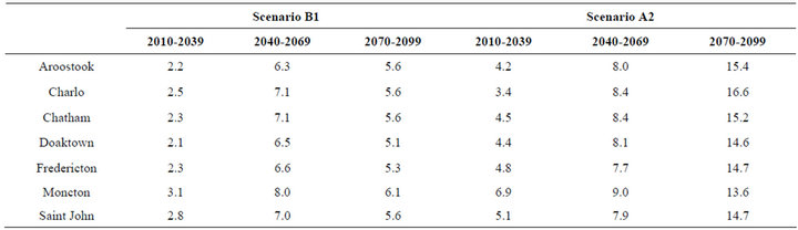
Table 4. Mean precipitation increase (%).
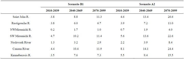
Table 5. Mean flow increase (%).
3.3. Floods and Droughts under Future Climate Change
Using the projected maximum and minimum river discharge for each station, events of different recurrence intervals were computed using the generalized extreme value (GEV) distribution. The parameters of the GEV for both high and low flows were estimated by the method of L-moments and the goodness of fit was assessed by the Anderson-Darling statistics. As such, the discharge of different recurrence intervals (high and low flows) was based on the maximum (and minimum) daily flow recorded each year.
The frequency analysis show that for all sites under investigation, the intensity and frequency of discharges will most likely increase in severity for both climate scenarios. The increase in high flows for low return floods (e.g., 2-year) was generally higher than higher return floods (e.g. 100-year). Depending on the scenario and the time slice used, the increases for low return floods was about 30% whereas increases was about 15% for higher return floods. Low flows showed increases of about 10% for low return droughts and about 20% for higher return droughts. These results show that floods will most likely experienced a greater change for low recurrence intervals (e.g., 2-year) whereas the droughts will be most affected for higher recurrence intervals
3.4. Regional Climate Index (RCI)
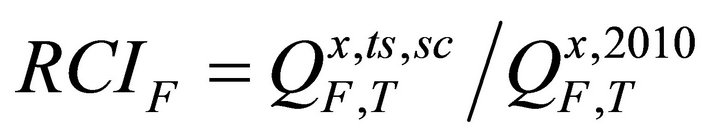
An important part of the design process using frequency analysis is the estimation of future change in floods or droughts under climate scenarios at a given site for specific return periods or recurrence intervals. This analysis was carried out through the application of regional regression models linking floods and droughts to their frequencies under future climate scenarios (B1 and A2). To accomplish this, a so-called Regional Climate Index (RCI) was introduced. This index was calculated by dividing future flows over historical flows, while maintaining the same characteristics parameters. This RCI can be expressed as follows:
For floods:
 (3)
(3)
For droughts:
 (4)
(4)
where  and
and  are the high or low flow at a site x, during time slice ts (2010-2039, 2040-2069 or 2070-2099), under scenario sc (B1 or A2), and for return period T.
  and
and  are the present time discharges at the same site x.
  and
and  are the regional climate index equations for floods and droughts defined as the mean ratio of discharges from the future time period relative to the historic period.
The RCIs were obtained through regression analyses using historical and future simulated floods (and low flows). In all cases, the coefficient of determination, R2, was about 0.99. These RCIs were developed for the whole province of New Brunswick, as future projections may contain some uncertainty at the site level. Tables 6 and 7 show the regression equations while Figures 3 and 4 show the RCI for floods and droughts for different return periods, for both scenarios B1 and A2 and for the different time periods. Figure 3 show that low return floods will increase by a factor of 1.3 to 1.4 whereas higher return floods will only increase by 1.05 to 1.1 (scenario B1). Under the scenario A2, the increase will be more important (1.35 to 1.56 for low return flood and 1.16 to 1.21 for high return floods). Figure 4 shows that droughts of low return periods will be less affected than higher return drought. However, in all cases, the severity of droughts will diminish, as an increase in flows is projected.
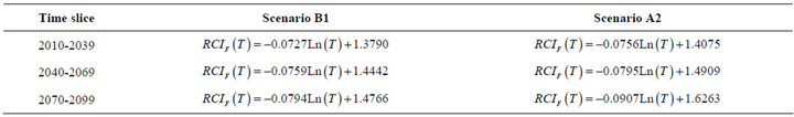
Table 6. Regional climate index equations for floods.
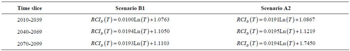
Table 7. Regional climate index equations for droughts.
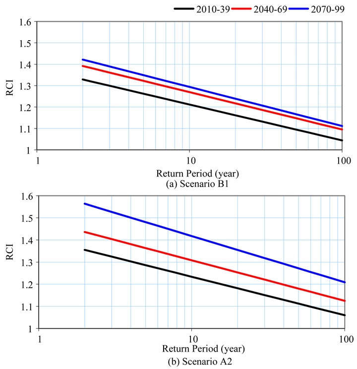
Figure 3. New Brunswick regional climate index curves for floods at time slices 2010-2039, 2040-2069, 2070-2099 under (a) scenario B1 (b) scenario A2.
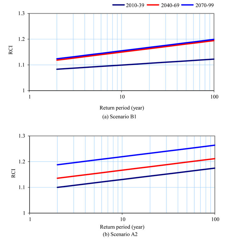
Figure 4. New Brunswick regional climate index curves for droughts at time slices 2010-2039, 2040-2069, 2070-2099 under a) scenario B1 b) scenario A2.
The future high and low flows in New Brunswick may therefore be estimated by:
For floods:
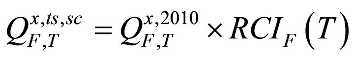 (5)
(5)
For droughts:
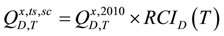 (6)
(6)
When expressed in percentage, it can be observed than future floods will most likely be higher than current floods by 30% - 40% (B1) or 35% - 55% (A2) for 2-year floods (Figure 3). Higher return floods (e.g. 100-year) are also expected to increase but not to the same extent as low return floods. For example, 100-year floods are projected to increase by 5% - 12% (B1) or 8% - 21% (A2). Figure 4 shows that future low flows would most likely be higher than current low flows. For instance, a 2-year low flow could be 9% - 12% higher under the B1 scenario or 10% - 19% higher under the A2 scenario. Higher return (e.g. 100-year) low flows would most likely be less severe than current conditions. The increase in low flow discharge is expected to be in the range of 11% 20% (B1) and 18% - 27% (A2).
4. Conclusion
Climate change will undoubtedly alter floods and droughts in New Brunswick. The success of industries (e.g., agriculture, forestry, fisheries and others) is intrinsically linked to climate and river flow, making New Brunswick particularly vulnerable to the impacts of climate change. Undoubtedly, these industries (among others) will be significantly affected by warmer and wetter climates with a potential shift in the availability of water during some seasons (e.g., summer and fall). Adaptation will be essential to maintaining the viability of some industries within the province. The hydrological response of seven catchments to two emission scenarios was simulated using artificial neural network (ANN). It was observed that air temperature in New Brunswick will increase by as much as 5.2˚C by 2100. This rate of warming is much greater than that observed in the 20th century but is consistent with that predicted by Parks Canada [1] and Houghton et al., [21] for the Atlantic Provinces.
As for precipitation, the mean annual precipitation showed an increase of 9% - 12% compared to current conditions.
The frequency analyses showed that flood magnitude would most likely increase by 11% - 21% towards the end of the century, depending on the emission scenario used. In term of low flows, the model is predicting a 20% - 26% increase towards the end of the century. This increase in low flow is most likely linked to the increase in precipitation in the future. Finally, future high and low flows were estimated by the introduction of a Regional Climate Index (RCI) for the province of New Brunswick. This RCI for floods and droughts was defined as the mean ratio of future discharge relative to the historic flow. As such, RCIs can used to estimate future floods and droughts conditions within the study area.
5. Acknowledgements
This study was funded by the New Brunswick Environmmental Trust Fund. The authors wish to thank anonymous reviewers for several helpful suggestions.
REFERENCES
- Parks Canada, “Air Quality, Climate Change and Canada’s National Parks,” Parks Canada, Natural Resources Branch, Air Issues Bulletin No. 100, Ottawa, 1999.
- H. G. Hengeveld, “Global Climate Change: Implication for Air Temperature and Water Supply in Canada,” Transactions of the American Fisheries Society, Vol. 119, No. 2, 1990, pp. 176-182. doi:10.1577/1548-8659(1990)119<0176:GCCIFA>2.3.CO;2
- Natural Resources Canada, “Climate Change Impacts and Adaptation: A Canadian Perspective,” Water Resources, Climate Change Impacts and Adaptation Directorate, Ottawa, 2002.
- C. K. Minns, R. G. Randall, E. M. P. Chadwick, J. E. Moore and R. Green, “Potential Impact of Climate Change on the Habitat and Population Dynamics of Juvenile Atlantic Salmon (Salmo salar) in Eastern Canada. Climate Change and Northern Fish Population,” Canadian Special Publications of Fisheries and Aquatic Sciences, 1995, pp. 699-708.
- D. Caissie,“Hydrological Conditions for Atlantic Salmon Rivers in the Maritime Provinces in 1997,” Canadian Stock Assessment SecretariatResearch Document, 1999.
- D. Caissie, “Hydrological Conditions for Atlantic Salmon Rivers in the Maritime Provinces in 1998,” Canadian Stock Assessment Secretariat Research Document, 1999.
- D. Caissie, “Hydrological Conditions for Atlantic salmon Rivers in 1999,” Canadian Stock Assessment Secretariat Research Document, 2000.
- Environment Canada and New Brunswick Department of Municipal Affairs and Environment, “Flood Frequency Analyses, New Brunswick, a Guide to the Estimation of Flood Flows for New Brunswick Rivers and Streams,” April 1987, p. 49.
- F. Aucoin, D. Caissie, N. El-Jabi and N. Turkkan, “Flood Frequency Analyses for New Brunswick Rivers,” Canadian Technical Report of Fisheries and Aquatic Sciences, 2011.
- Environment Canada and New Brunswick Department of the Environment, “Low Flow Estimation Guidelines for New Brunswick,” Inland Waters Directorate, Environment Canada, Dartmouth, NS and Water Resources Planning Branch, New Brunswick Department of the Environment, Fredericton, 1990.
- D. Caissie, L. LeBlanc, J. Bourgeois, N. El-Jabi and N. Turkkan, “Low Flow Estimation for New Brunswick Rivers,” Canadian Technical Report of Fisheries and Aquatic Sciences, 2011.
- J. Alcamo, A. Bouwman, J. Edmonds, A. Grübler, T. Morita and A. Sugandhy, “An Evaluation of the IPCC IS92 Emission Scenarios,” In J. T. Houghton, L. G. Meira Filho, J. Bruce, H. Lee, B. A. Callander, E. Haites, N. Harris and K. Maskell, Eds., Radiative Forcing of Climate Change and an Evaluation of the IPCC IS92 Emission Scenarios, Cambridge University Press, Cambridge, 1995, pp. 233-304.
- N. Nakicenovic, A. Grubler, H. Ishitani, T. Johansson, G. Marland, J. R. Moreira and H.-H. Rogner, “Energy Primer in Climate Change 1995,” In: R Watson, M. C. Zinyowera and R. Moss, Eds., Impacts, Adaptations and Mitigation of Climate Change: Scientific Analysis, Cambridge University Press, Cambridge, UK, 1996.
- D. Caissie and S. Robichaud, “Towards a Better Understanding of the Natural Flow Regimes and Streamflow Characteristics of Rivers of the Maritime Provinces,” Canadian Technical Report of Fisheries and Aquatic Sciences, 2009.
- C. Prudhomme, N. Reynard and S. Crooks, “Downscaling from Global Climate Models for Flood Frequency Analysis: Where Are We Now?” Hydrological Processes, Vol. 16, No. 6, 2002, pp. 1137-1150. doi:10.1002/hyp.1054
- N. Turkkan, N. El-Jabi and D. Caissie,“Floods and Droughts under Different Climate Change Scenarios in New Brunswick,” Canadian Technical Report of Fisheries and Aquatic Sciences, 2011.
- H. Fowler and C. Kilsby, “Using Regional Climate Model Data to Simulate Historical and Future River Flows in Northwest England,” Climatic Change, Vol. 80, No. 3, 2007, pp. 337-367. doi:10.1007/s10584-006-9117-3
- R. S. Govindaraju, “Artificial Neural Networks in Hydrology. I: Preliminary Concepts,” Journal of Hydrologic Engineering, Vol. 5, No. 2, 2000, pp.115-123. doi:10.1061/(ASCE)1084-0699(2000)5:2(115)
- R. S. Govindaraju, “Artificial Neural Networks in Hydrology. II: Hydrologic Application,” Journal of Hydrologic Engineering, Vol. 5, No. 2, 2000, pp. 124-137. doi:10.1061/(ASCE)1084-0699(2000)5:2(124)
- D. Bastarache, N. El-Jabi, N. Turkkan and T. A. Clair. “Predicting Conductivity and Acidity for Two Small Streams Using Learning Networks,” Canadian Journal of Civil Engineering, Vol. 24, 1997, pp. 1030-1039. doi:10.1139/cjce-24-6-1030
- J. T. Houghton, D. Ding, J. Griggs, M. Noguer, P. J. Z. van der Linden and D. Xiaosu, “Climate Change 2001: The Scientific Basis,” Contribution of Working Group I to the Third Assessment Report of the Intergovernmental Panel on Climate Change (IPCC), Cambridge University Press, Cambridge, 2001.