International Journal of Modern Nonlinear Theory and Application
Vol.04 No.02(2015), Article ID:57217,14 pages
10.4236/ijmnta.2015.42009
Velocity Projection with Upwind Scheme Based on the Discontinuous Galerkin Methods for the Two Phase Flow Problem
Jiangyong Hou1,2, Wenjing Yan1,2*, Jie Chen1,2
1School of Mathematics and Statistics, Xi’an Jiaotong University, Xi’an, China
2Center for Computational Geosciences, Xi’an Jiaotong University, Xi’an, China
Email: *wenjingyan@mail.xjtu.edu.cn
Copyright © 2015 by authors and Scientific Research Publishing Inc.
This work is licensed under the Creative Commons Attribution International License (CC BY).
http://creativecommons.org/licenses/by/4.0/


Received 20 March 2015; accepted 12 June 2015; published 17 June 2015
ABSTRACT
The upwind scheme is very important in the numerical approximation of some problems such as the convection dominated problem, the two-phase flow problem, and so on. For the fractional flow formulation of the two-phase flow problem, the Penalty Discontinuous Galerkin (PDG) methods combined with the upwind scheme are usually used to solve the phase pressure equation. In this case, unless the upwind scheme is taken into consideration in the velocity reconstruction, the local mass balance cannot hold exactly. In this paper, we present a scheme of velocity reconstruction in some H(div) spaces with considering the upwind scheme totally. Furthermore, the different ways to calculate the nonlinear coefficients may have distinct and significant effects, which have been investigated by some authors. We propose a new algorithm to obtain a more effective and stable approximation of the coefficients under the consideration of the upwind scheme.
Keywords:
Velocity Projection, Upwind Scheme, Penalty Discontinuous Galerkin Methods, Two Phase Flow in Porous Media

1. Introduction
In the context of some fields, such as modeling and simulation of fluid flows in petroleum or groundwater reservoirs, the studies of processes of the simultaneous flow of two or more fluid phases within a porous medium are of great significance. In this paper, we consider the cases of two-phase flow where the fluids are immiscible. A large number of methods, which are based on the finite difference (FD), the finite volume (FV) or the finite element (FE) methods, have been developed to deal with the two-phase flow problem. As is well known, no matter which kind of numerical methods is used, the upwind scheme is of great significance in the approximation of some problems such as the convection dominated problem, the two-phase flow problem, and so on.
To achieve stable numerical computations in the simulation of two-phase flow problem, an accurate approximation of the flux is one of the most important and desirable ingredients. If we use Penalty Discontinuous Galerkin (PDG) methods to discretize the pressure equation, like in [1] -[3] , both the pressure and saturation equations will be discritized by the PDG methods, and a process of reconstruction of the velocity needs to be done after the pressure equation is solved. In [2] , an average total velocity was post processed by substituting the piecewise constants of pressure gradient and saturation gradient into the velocity-pressure expression directly. Actually such reconstructed velocity, on some level, belongs to the lowest order Raviart-Thomas finite element space. In [4] , a post-processed total velocity is reconstructed in the Brezzi-Douglas-Marini (BDM) finite element spaces. But it needs that the degree of the polynomial is more than one, that is, using the linear approximation in DG method is not enough to reconstruct a velocity in BDM1 space. A more stable and accurate reconstruction was developed in [1] , in which the velocity reconstructed from the piecewise linear pressures could even belong to the first-order Raviart-Thomas finite element space. However, all the reconstructions mentioned above didn’t consider the upwind scheme, which was basically used in the discretization of the equations. The property of the local mass conservation is crucial in porous media flow and transport problems. The upwind scheme has direct effect on the local mass conservation of the reconstructed velocity. We found that unless the upwind scheme and penalty terms which are used in the discretization of the two-phase flow problem are considered together into the velocity reconstruction, the error of the local mass conservation cannot reach a satisfactory level. In this paper, we present a scheme of velocity reconstruction in some H(div) spaces [5] with considering the upwind scheme totally.
The different ways to calculate the nonlinear coefficients may have distinct and significant effects, which have been investigated by some authors. For the approximation of the coefficients, we extend the one used in [6] to that each coefficient in element K is evaluated as the average of the upwind value on . This improves the stability of the numerical scheme even when an explicit scheme is used. In contrast with the explicit scheme described in [2] , our explicit PDG scheme with this special approximation of coefficients can not only get rid of the extra penalties from the pressure equation but also have a robust performance in the heterogeneous media.
The rest of the article is organized as follows: In addition to the introduction and conclusion, we divide the text of this document into four parts. Section 2 is the first part and consists of two subsections, in which we introduce governing equations of two-phase flow problem and the corresponding interface conditions in Subsections 2.1 and 2.2 respectively. The second part, Section 3, comes in four subsections. In Subsection 3.1, the upwind average approximations of coefficients are introduced. In Subsections 3.2 and 3.3, the PDG methods are used for the pressure equation and the velocity reconstruction is presented respectively. In Subsection 3.4, the PDG methods are used for the saturation equation. The third part, Section 4, consists of two subsections. In Subsections 4.1 and 4.2, we introduce all the possible projection schemes with respect to the velocity reconstruction and the scheme without any explicit projections. In the last part, Section 5, several numerical examples in two dimensions are provided.
2. Problem Model
2.1. Mathematical Formulation
We consider two immiscible incompressible fluids in porous media and there is no mass transfer between the phases. Various and alternative model equations for two-phase flow problem can be found in reference [7] . Here we use the phase formulation for which the primary variables are wetting phase pressure and saturation ( and
and ), and in the absence of gravity and sink/source term we have:
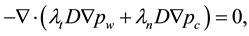 (1)
(1)
![]() (2)
(2)
where the denotations and meanings of each coefficient and their relationships are defined as follows: D is the absolute permeability tensor and is discontinuous in heterogeneous media; ![]() denotes the porosity of the medium;
denotes the porosity of the medium; ![]() is the capillary pressure;
is the capillary pressure;![]() ,
, ![]() and
and ![]() are wetting, nonwetting and total mobility respectively;
are wetting, nonwetting and total mobility respectively; ![]() is the fractional flow;
is the fractional flow; ![]() and
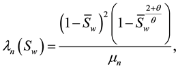
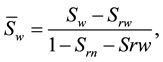
and ![]() are the gradient operator and divergence operator respectively. We will use the Brooks-Corey model [8] throughout this paper, in which some of these coefficients are non-linear functions defined below:
are the gradient operator and divergence operator respectively. We will use the Brooks-Corey model [8] throughout this paper, in which some of these coefficients are non-linear functions defined below:
![]() (3)
(3)
 (4)
(4)
 (5)
(5)
 (6)
(6)
 (7)
(7)
where  is the entry pressure needed for the wetting phase to enter large pores which are completely filled with the non-wetting phase;
  and
and  are the non-wetting and wetting phase viscosity;
  is the parameter associated with pore size distribution;
  and
and  are the residual saturation.
Some notations for the mesh are given below:  is the domain;
  is the boundary of the domain;
  is the partition of
 ; K is the finite element in
 ;
;  is the edges of element K;
  {e: all edges in
  }, is the set of all edges contained in
 ;
;  is the set of all interior edges contained in
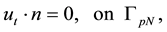
 . The Equations (1) and (2) are subject to appropriate initial and boundary conditions to close the system. Here we give two feasible sets of boundary conditions: one is the Mixed-Neumann boundary condition as in [2] ,
 (8)
(8)
 (9)
(9)
 (10)
(10)
 (11)
(11)
and the other is Neumann-Drichlet boundary condition used in [9] ,
 (12)
(12)
 (13)
(13)
 (14)
(14)
 (15)
(15)
The whole boundary of the porous medium domain  is divided into three mutually disjoint parts: the inflow, noflow, and outflow boundaries (
 ,
,  ,
, ), respectively. In the case of Neumann-Drichlet boundary condition,
  and
and  occupy the outflow boundary,
  and
and  occupy the inflow and no-flow boundaries such that
  on inflow boundary and
  on no-flow boundary. In the case of mixed- Neumann boundary condition,
  occupies the inflow and outflow boundaries,
  occupies the no-flow boundary,
  occupies the inflow boundary, and
  occupies the no-flow and outflow boundaries.
2.2. Interface Conditions
In order to test the barrier effect phenomenon of two phase flow, the nonlinear interface condition discussed in [1] [6] [10] -[13] will be introduced here. Following [9] , we assume an initially fully water saturated domain  with an interface
  between two different sands, and the oil is injected from the inflow part of boundary
 , see Figure 1. In addition, we assume that
  stands the coarse sand and
  is the fine sand.
The process of the phenomenon is described briefly below. First, oil approaches the material interface but cannot penetrate it and begin to accumulate. In this case, only water pressure  is continuous on the interface, capillary pressure
  and saturation
  are discontinuous and satisfy:
 (16)
(16)
Then, when more and more oils accumulate at the interface and the capillary pressure on the coarse side exceeds the entry pressure of the other side , the oils begin to penetrate and enter the fine sand. At this time, both
  and
and  are continuous, but saturation
  is still discontinuous and satisfies:
 (17)
(17)
We note that a critical point of saturation can be found when the capillary pressure on coarse side increases to the value equivalent to the threshold pressure on fine side. That is, deducing from  we have,
 (18)
(18)
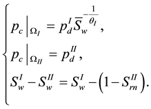
This point will be used to judge whether the nonwetting phase can or cannot penetrate the material interface. So the interface conditions can be rewritten in the form below. For capillary pressure,
 (19)
(19)
and for wetting phase saturation,
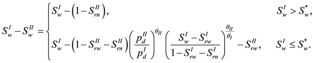 (20)
(20)
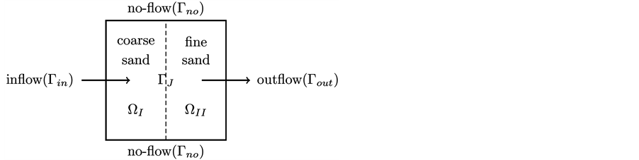
Figure 1. The interface (dashed line) between two subdomains with different rock properties.
Condition (20) is the same as that described in [1] except that the wetting phase (instead of the nonwetting phase) is used as the saturation variable. Moreover, (19) is only written for the capillary pressure and not for the wetting phase pressure, since the variable  is always continuous in the problem discussed. Noting that if the sub-domain
  has a finer texture than
 , all the relationship above can be treated in a similar manner with superscript
  and
and  reversed.
3. Discrete Schemes
3.1. Approximation of Coefficients
For the approximation of coefficients,we extend the one used in [6] . Let  denote any coefficients waiting for some proper approximations. Firstly we recall the original way to approximate the coefficients,
 (21)
(21)
The approach described in [6] is,
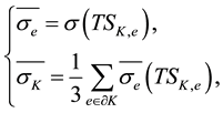 (22)
(22)
where  denotes the mean water saturation on the edge e of the element K, see [6] for more details. Now it is extended to the following one,
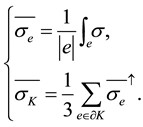 (23)
(23)
where the upwind value of the side average on the interior edge is considered. The quantity  is called the upwind flux which is done with respect to the normal component of the total velocity
 , such that for all
 ,
,
 (24)
(24)
where the normal vector  points from
  to
to . Throughout this paper, all the coefficients on element K and edge e are calculated by the upwind averaged constant and the integral average constant which are described in (23).
3.2. Pressure Approximation with PDG
In this section we apply the Penalty Discontinuous Galerkin (PDG) methods [14] such as Nonsymmetric Interior Penalty Galerkin (NIPG) to the pressure Equation (1). Some notations for DG methods are defined:
 (25)
(25)
![]() (26)
(26)
![]() (27)
(27)
where ![]() are the restrictions of v on two adjacent elements
are the restrictions of v on two adjacent elements ![]() respectively.
respectively.
The pressure Equation (1) discretized by PDG reads as follows.
![]() (28)
(28)
Indeed, the PDG methods are only applied to the wetting-phase pressure term, for the capillary pressure term a traditional DG method with the upwind scheme is used.
3.3. Velocity Reconstruction
After solving the discrete pressure Equation (28), the total velocity will be reconstructed in the lowest-order Raviart-Thomas space![]() , the first-order Raviart-Thomas space
, the first-order Raviart-Thomas space ![]() and the first-order Brezzi-Douglas- Marini space
and the first-order Brezzi-Douglas- Marini space ![]() respectively, refer to [5] for more details about those spaces. The main idea of the reconstruction in the current section follows the one depicted in [1] , and we will extend it to the situation that the discretization of the pressure equation contains an upwind scheme.
respectively, refer to [5] for more details about those spaces. The main idea of the reconstruction in the current section follows the one depicted in [1] , and we will extend it to the situation that the discretization of the pressure equation contains an upwind scheme.
A proper reconstruction of velocity stems from the local mass conservation law as shown in the following description. Firstly, we recast the variational Equation (28) on element K into two parts as follows,
![]() (29)
(29)
![]() (30)
(30)
Combing (29) and (30), it is easily seen that the local mass is conserved,
![]() (31)
(31)
where ![]() and
and ![]() are the sink and source terms which are zeros here. Noting that if the edge e belongs to both
are the sink and source terms which are zeros here. Noting that if the edge e belongs to both ![]() and
and ![]() on the right hand side of Equations (29) and (30),
on the right hand side of Equations (29) and (30), ![]() is equal to
is equal to ![]() and the sign
and the sign ![]() is determined by the direction of
is determined by the direction of![]() , for example, the sign is positive when
, for example, the sign is positive when ![]() is the outer normal vector with respect to
is the outer normal vector with respect to![]() .
.
Secondly, using (29) and (30) as the degree of freedom for some H(div) spaces, the total velocity will be obtained as some appropriate projections or interpolations in these spaces. In order to have a proper interpolation in![]() ,
, ![]() and
and ![]() spaces, we should specify a set of degree of freedom (DOF) for these H(div) spaces and a corresponding set of basis functions. If let v be any constant in the polynomial space of degree zero
spaces, we should specify a set of degree of freedom (DOF) for these H(div) spaces and a corresponding set of basis functions. If let v be any constant in the polynomial space of degree zero![]() , (29) will vanish and (30) will become the
, (29) will vanish and (30) will become the ![]() space’s DOF which is the integral of the normal component of velocity on each edge. Correspondingly, the set of basis functions for
space’s DOF which is the integral of the normal component of velocity on each edge. Correspondingly, the set of basis functions for ![]() on the reference element is,
on the reference element is,
![]() (32)
(32)
where ![]() is the area of the reference element
is the area of the reference element ![]() and
and ![]() is one of its the vertices.
is one of its the vertices.
Let ![]() and
and ![]() be any functions in the space of polynomial of degree one
be any functions in the space of polynomial of degree one![]() , then (29) and (30) become the DOFs for
, then (29) and (30) become the DOFs for![]() . The corresponding basis functions for
. The corresponding basis functions for ![]() space on the reference elements are,
space on the reference elements are,
![]()
![]()
![]()
![]()
Let ![]() be any functions in
be any functions in ![]() polynomial space, thus the basis functions of
polynomial space, thus the basis functions of ![]() can be obtained in a similar manner except that (29) is not used. All the DOFs for
can be obtained in a similar manner except that (29) is not used. All the DOFs for ![]() are just defined on the edges of element, so only (30) is used to determine the basis functions. The corresponding basis functions for
are just defined on the edges of element, so only (30) is used to determine the basis functions. The corresponding basis functions for ![]() are,
are,
![]()
![]()
![]()
It is noted that the choice of DOFs for the ![]() and
and ![]() spaces is not unique, for example, the half-edge integral of the normal components of velocity is also available and applicable.
spaces is not unique, for example, the half-edge integral of the normal components of velocity is also available and applicable.
3.4. Saturation Approximation
The spatial discretization of the saturation equation is similar to that of the pressure equation given in (28). The diffusion term of the saturation equation is discretized by the PDG methods, and the advective term is discretized by a traditional DG method with using the upwind scheme. An Euler scheme in time is used. The saturation Equation (2) equipped with Mixed-Neumann boundary conditions (8)-(11) could be written as:
![]() (33)
(33)
The variational form in terms of Neumann-Dirichlet boundary conditions (12)-(15) reads:
![]() (34)
(34)
where ![]() is the interface condition of saturation described in (20).
is the interface condition of saturation described in (20).
4. Feasible Projections of the Discrete Strategies
4.1. DDG Methods with Some Other Projections
The abbreviation DDG means that DG methods are used for both pressure and saturation equations. For a clear comparison in the numerical experiments, we list all the possible and feasible projections below. Firstly, we denote RT(1) (or BDM(1)) as the the velocity space projected into RT (or BDM) space by (29) and (30). Secondly, RT(2) (or BDM(2)) means the projection into RT (or BDM) space with considering the upwind scheme but without the penalty term,
![]() (35)
(35)
![]() (36)
(36)
Thirdly, for ![]() (or
(or![]() ), it means the projection with considering the penalty term but without the upwind scheme,
), it means the projection with considering the penalty term but without the upwind scheme,
![]() (37)
(37)
![]() (38)
(38)
At last, for ![]() (or
(or![]() ), it means the projection without considering both the penalty term and the upwind scheme,
), it means the projection without considering both the penalty term and the upwind scheme,
![]() (39)
(39)
![]() (40)
(40)
As indicated in introduction, for all DDG methods the velocity derived by the projection ![]() (or
(or![]() ) preserves the local mass conservation property best, which will shown in the numerical examples.
) preserves the local mass conservation property best, which will shown in the numerical examples.
4.2. DDG Method without Explicit Projections
In [2] the velocity is used directly as the combination of the gradient of the solutions and coefficients, as follows,
![]() (41)
(41)
![]() (42)
(42)
where the average of the total velocity is used in the interior edges. Although it doesn’t use any projections explicitly, the velocities constructed from (41) and (42) are some kind of implicit projections into ![]() space. The velocity derived from (41) and (42) is close to the velocity projection in
space. The velocity derived from (41) and (42) is close to the velocity projection in ![]() space which is constructed by (39) and (40). But their value in each element is different. Furthermore, the DDG method with using the velocity reconstruction presented in this subsection has certain differences in contrast to what proposed in [2] , which are reflected in two aspects below:
space which is constructed by (39) and (40). But their value in each element is different. Furthermore, the DDG method with using the velocity reconstruction presented in this subsection has certain differences in contrast to what proposed in [2] , which are reflected in two aspects below:
1) The variational form of the saturation equation doesn’t incorporate any additional penalties from the pressure equation.
2) The approximations of the coefficients are totally different.
5. Numerical Examples
In this section, we present some computer experiments to examine the proposed methods on two dimensional spaces. Both two boundary conditions with different types are used in the examination of all the methods. In tests 1 and 2 we consider the displacement of the non-wetting phase by the wetting phase, which is similar to the so called quarter-five spot problem introduced in [2] . In test 3 we consider the displacement of the wetting phase by the non-wetting phase which is used to simulate the barrier effect in [9] . The domains used in the experiments are the square ![]() with two corners be cut off, and for the mesh used in the discontinuous problem a small square with different rock property is fixed inside the domain, see Figure 2(a) and Figure 2(b). In each test, we use the Nonsymmetric Interior Penalty Galerkin (NIPG) method with the penalty parameters
with two corners be cut off, and for the mesh used in the discontinuous problem a small square with different rock property is fixed inside the domain, see Figure 2(a) and Figure 2(b). In each test, we use the Nonsymmetric Interior Penalty Galerkin (NIPG) method with the penalty parameters![]() ,
, ![]() and
and![]() . In order to prevent the oscillations, a slope limiter procedure described in [15] is used.
. In order to prevent the oscillations, a slope limiter procedure described in [15] is used.
If considering the mixed-Neumann type boundary (8)-(9) for the saturation equation, the following initial and boundary conditions are used:
![]() (43)
(43)
![]() (44)
(44)
![]() (45)
(45)
![]() (46)
(46)
![]() (a) (b)
(a) (b)
Figure 2. Meshes used in the experiments. (a) quarter-five spot mesh used in homogeneous medium; (b) quarter- five spot mesh used in discontinuous media.
![]() (47)
(47)
![]() (48)
(48)
When the Neumann-Dirichlet type boundary (12)-(13) is used for the saturation equation, the following initial and boundary conditions are considered:
![]() (49)
(49)
![]() (50)
(50)
![]() (51)
(51)
![]() (52)
(52)
![]() (53)
(53)
![]() (54)
(54)
![]() (55)
(55)
The parameters including rock and fluid properties used in the simulation are summarized in Table 1.
5.1. Test 1
In test 1, we examine the property of the local mass conservation law. For this purpose, we solve the so-called quarter-five spot problem on a homogeneous medium and check the numerical local mass of the reconstructed velocity. All the projection methods discussed above will be used and compared. The domain used in the experiment is the square ![]() with two corners be cut off, see Figure 2(a). The initial and boundary conditions (43)-(48) is used. The parameters with respect to the rock property and Brooks-Corey model are listed in Table 1, Test 1. In Figure 2(a), the spot at the left bottom is the inflow boundary
with two corners be cut off, see Figure 2(a). The initial and boundary conditions (43)-(48) is used. The parameters with respect to the rock property and Brooks-Corey model are listed in Table 1, Test 1. In Figure 2(a), the spot at the left bottom is the inflow boundary![]() , the outflow boundary
, the outflow boundary ![]() is located at the right top corner, the rest of the boundary is the noflow boundary
is located at the right top corner, the rest of the boundary is the noflow boundary![]() . To make sure that the water front stays inside the domain, the final time is set to T = 160 s. We use a constant time step, and the ratio of the time step to the space step’s square is about
. To make sure that the water front stays inside the domain, the final time is set to T = 160 s. We use a constant time step, and the ratio of the time step to the space step’s square is about![]() . We use
. We use ![]() to denote the DDG method without
to denote the DDG method without

Table 1. Parameters used in the numerical simulations.
explicit projections. Since there is no sink and source terms the exact local mass is zero on each elements, that is,
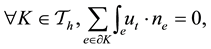 where
where  is the outward unit normal vector to
 . Thus we can easily define the
errors of the local mass conservation under the vector norms  and
and  which are respectively
 (56)
(56)
The errors of the local mass conservation at selected times are listed in Table 2 and Table 3.
5.2. Test 2
In this test, we show the numerical solutions solved by our scheme with using projection  in a homogeneous media. For the results with using projection
  and
and , they are similar with using
  so are omitted. The mesh used in test 2 is the same as the previous test.The initial and boundary conditions (43)-(48) are used in this test. To make sure that the water front stays inside the domain, the final time is set to T = 180 s. A constant time step is used, and the ratio of the time step to the space step’s square is about
 . The parameters of rock property and Brooks-Corey model are listed in Table 1, Test 2. The contours of wetting phase saturation in the homogeneous medium at selected times are presented in Figure 3.
5.3. Test 3
In the last test, we examine our scheme in a discontinuous media. We assume that the domain used here is initially fully water saturated and with the interfaces between two different sands, see Figure 4.  is the fine sand and
  is the coarse sand, so the oil-trapped phenomenon will appear on the interfaces
  see Figure 4. The critical point in (19) is
 , and the oil will penetrate the interface
  when
when . The mesh
Table 2. Numerical errors of the local mass conservation in test 1 at times t = 40 s and t = 80 s.
Table 3. Numerical errors of the local mass balance in test 1 at times t = 120 s and t = 160 s.
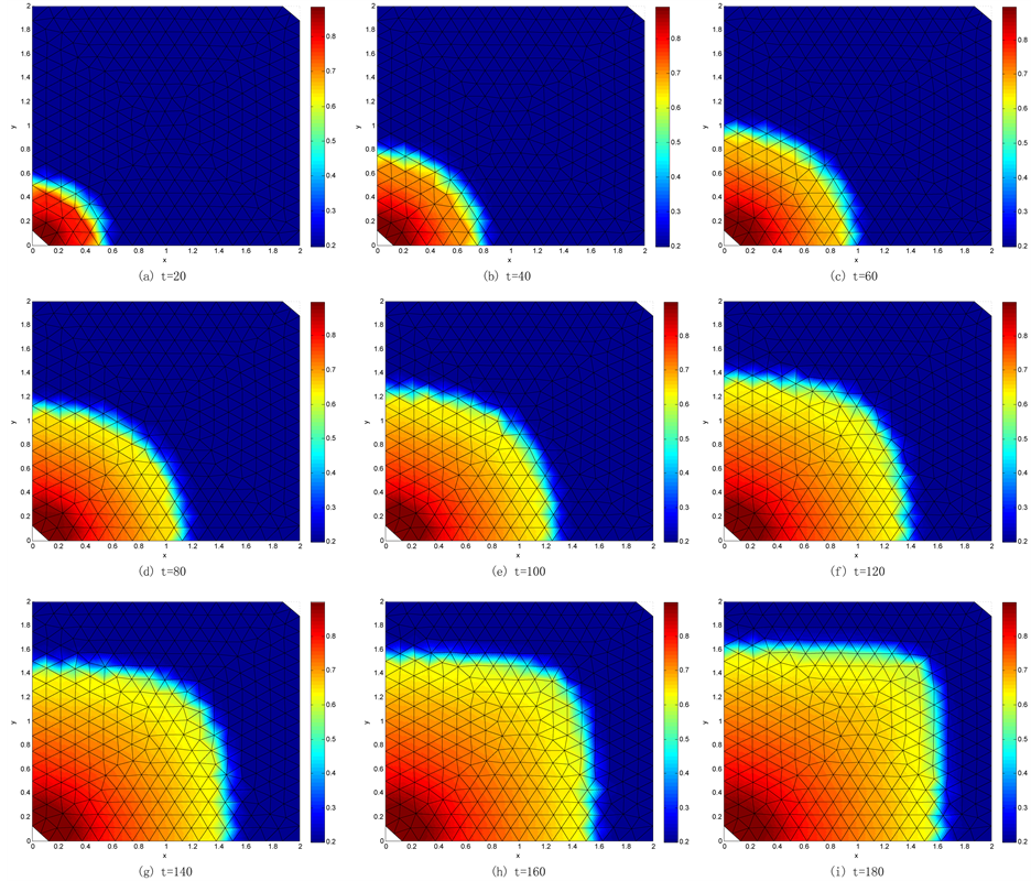
Figure 3. The contours of wetting phase saturation in the homogeneous medium at selected times in the Test 2.
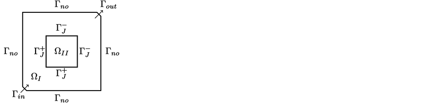
Figure 4. Discontinuous quarter-five spot problem.
used in this test is Figure 2(b). The initial and boundary conditions (49)-(55) are used in this test. The initial and boundary conditions (49)-(55) are used in this test. To make sure that the water front stays inside the domain, the final time is set to T = 200 s. A constant time step is used, and the ratio of the time step to the space step’s square is about . The parameters of rock property and Brooks-Corey model are listed in Table 1, Test 3. When the oil flows from coarse sand to fine sand with the injection of oil from the inflow boundary
 , more and more oil approaches and accumulates at the front of the interface of the fine sand. When the accumulation reaches a critical point, that is, when the capillary pressure at the coarse side of the interface is greater than at the fine side, the accumulated oil will penetrate the interface and enter the fine sand area. By contrast, in
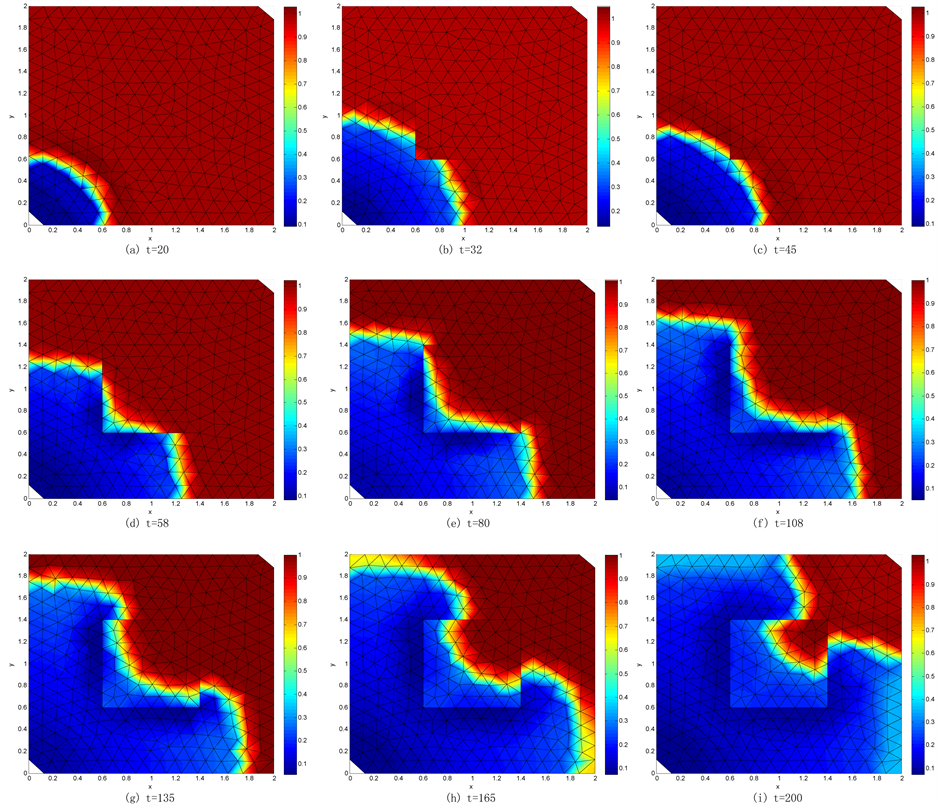
Figure 5. The contours of wetting phase saturation in the discontinuous media at selected times in the Test 3.
the reversed direction the oil immediately penetrate the interface, that is, the oil-trapped phenomenon will not happen if the oil flows from fine sand to coarse sand. The contours of wetting phase saturation in the discontinuous media at selected times are presented in Figure 5.
6. Conclusion
The velocities reconstructed from projections 
 and
and  are much better to preserve the local mass conservation property than the others. That is, the velocity reconstruction with the projection that considers both the upwind scheme and penalty term can best preserve the local mass conservation property. The approximation of the coefficient (23) is very essential to the stability of all the DDG methods. Instead of (23), if the approximation of coefficient (21) is used, the variational form of the saturation equation has to incorporate additional penalties from the pressure equation; otherwise the scheme will be unstable.
Funding
The work is supported by the National Natural Science Foundation of China (No.11371288 and No.11401467).
References
- Ern, A., Mozolevski, I. and Schuh, L. (2010) Discontinuous Galerkin Approximation of Two-Phase Flows in Heterogeneous Porous Media with Discontinuous Capillary Pressures. Computer Methods in Applied Mechanics and Engineering, 199, 1491-1501. http://dx.doi.org/10.1016/j.cma.2009.12.014
- Klieber, W. and Rivière, B. (2006) Adaptive Simulations of Two-Phase Flow by Discontinuous Galerkin Methods. Computer Methods in Applied Mechanics and Engineering, 196, 404-419. http://dx.doi.org/10.1016/j.cma.2006.05.007
- Mozolevski, I. and Schuh, L. (2013) Numerical Simulation of Two-Phase Immiscible Incompressible Flows in Heterogeneous Porous Media with Capillary Barriers. Journal of Computational and Applied Mathematics, 242, 12-27. http://dx.doi.org/10.1016/j.cam.2012.09.045
- Bastian, P. and Rivière, B. (2003) Superconvergence and H(div) Projection for Discontinuous Galerkin Methods. International Journal for Numerical Methods in Fluids, 42, 1043-1057. http://dx.doi.org/10.1002/fld.562
- Brezzi, F. and Fortin, M. (1991) Mixed and hybrid finite element methods. Springer, New York. http://dx.doi.org/10.1007/978-1-4612-3172-1
- Nayagum, D., Schäfer, G. and Mosé, R. (2004) Modelling Two-Phase Incompressible Flow in Porous Media Using Mixed Hybrid and Discontinuous Finite Elements. Computational Geosciences, 8, 49-73. http://dx.doi.org/10.1023/B:COMG.0000024446.98662.36
- Chen, Z.X., Huan, G.R. and Ma, Y.L. (2006) Computational Methods for Multiphase Flows in Porous Media. SIAM, Philadelphia. http://dx.doi.org/10.1137/1.9780898718942
- Brooks, R.H. and Corey, A.T. (1964) Hydraulic Properties of Porous Media. Colorado State University, Fort Collins.
- Fučk, R. and Mikyška, J. (2011) Mixed-Hybrid Finite Element Method for Modelling Two-Phase Flow in Porous Media. Journal of Math-for-Industry, 3, 9-19.
- Hoteit, H. and Firoozabadi, A. (2008) Numerical Modeling of Two-Phase Flow in Heterogeneous Permeable Media with Different Capillarity Pressures. Advances in Water Resources, 31, 56-73. http://dx.doi.org/10.1016/j.advwatres.2007.06.006
- Enchéry, G., Eymard, R. and Michel, A. (2006) Numerical Approximation of a Two-Phase Flow Problem in a Porous Medium with Discontinuous Capillary Forces. SIAM Journal on Numerical Analysis, 43, 2402-2422. http://dx.doi.org/10.1137/040602936
- Cancès, C. (2009) Finite Volume Scheme for Two-Phase Flow in Heterogeneous Porous Media Involving Capillary Pressure Discontinuities. ESAIM: Mathematical Modelling and Numerical Analysis, 43, 973-1001. http://dx.doi.org/10.1051/m2an/2009032
- Cancès, C., Gallouët, T. and Porretta, A. (2009) Two-Phase Flows Involving Capillary Barriers in Heterogeneous Porous Media. Interfaces and Free Boundaries, 11, 239-258. http://dx.doi.org/10.4171/IFB/210
- Rivière, B. (2008) Discontinuous Galerkin Methods for Solving Elliptic and Parabolic Equations: Theory and Implementation. SIAM, Philadelphia. http://dx.doi.org/10.1137/1.9780898717440
- Chavent, G. and Jaffré, J. (1986) Mathematical Models and Finite Elements for Reservoir Simulation. Studies in Mathematics and Its Applications. North-Holland, Amsterdam.
NOTES

*Corresponding author.