ABSTRACT

This paper presents a complete integrability condition for fully rheonomous affine constraints in terms of the rheonomous bracket. We first define fully rheonomous affine constraints and develop geometric representation for them. Next, the rheonomous bracket is explained and some properties of it are derived. We then investigate a necessary and sufficient condition on complete integrability for the fully rheonomous affine constraints based on the rheonomous bracket as an extension of Frobenius’ theorem. The effectiveness and the availability of the new results are also evaluated via an example.

1. Introduction

Many studies on nonholonomic systems [1-3] and subRiemannian geometry [4,5] have been done in the research fields of mathematics, control theory, and robotics and so on so far. Especially, the class of linear constraints:, , , which is one of most fundamental classes of constraints, has been mainly studied. The class of the linear constraints covers wide-ranging mechanical systems such as mobile and acrobatic robots, however, there also exist wider classes of constraints.

The author has focused and researched affine constraints: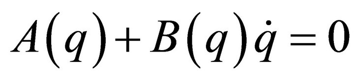, , which form a wider class of constraints than the linear constraints, from the viewpoints of mathematics and control theory. The affine constraints can be found in mechanical systems such as space robots with initial angular momenta, a ball on a rotating table, a ship on a running river, and so on. Especially, in [6,7], we investigated integrability and nonintegrability of the affine constraints and derived some judgment conditions. Moreover, as an extension of these studies, we dealt with A-rheonomous affine constraints: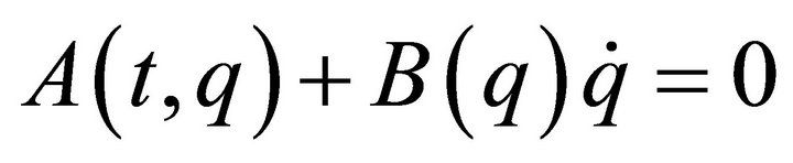, which contain the time variable explicitly only in [8-10]. Note that in analytical mechanics, the terminology “rheonomous” means “time-varying,” and the opposite word of it is “scleronomous”. These results have made it possible to treat such constraints systematically, however, we are still interested in fully rheonomous affine constraints: as a much wider class of constraints than the A-rheonomous affine constraints. If the extension of the results to the fully rheonomous affine constraints, the range of applications will enlarge further.

In this paper, we aim at derivation of some properties on the rheonomous bracket and an integrability condition for the fully rheonomous affine constraints as an extension of Frobenius’ theorem for the linear constraints [11-14]. The organization of this paper is as follows. In Section 2, we first define the fully rheonomous affine constraints and introduce their geometric representation. Next, in Section 3, we explain the rheonomous bracket and investigate its some properties. We then derive a necessary and sufficient condition on complete integrability for the fully rheonomous affine constraints in terms of the rheonomous bracket in Section 4. Finally, Section 5 shows an example for verification of the effectiveness and the availability of the new results.

2. Fully Rheonomous Affine Constraints

In this section, we first give the definition of fully rheonomous affine constraints and introduce their geometric representation. Denote the time variable by and a time interval by. Let be an -dimensional configuration manifold and

be a local coordinate of. Associated with, we refer as a tangent vector field. A set of of differential equations in the form:

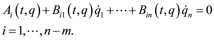(1)

is called fully rheonomous affine constraints. Note that all the coefficients explicitly depend on the time variable. We now rewrite (1) as

(2)

where a rheonomous affine term is a vector-valued function whose -th entry is, and a velocity coefficient matrix is a matrixvalued function whose -th entry is. We here assume the following sufficient condition on independency of the fully rheonomous affine constraints (2):

. (3)

Next, we shall introduce geometric representation of the fully rheonomous affine constraints (2). From (1), we can see that the row vectors of in (2) are independent of each other. Hence, we consider vector fields which are independent of each other and annihilators of the row vectors of, and denote them by as time-varying vector fields on. Furthermore, we also denote a space spanned by, that is, a time-varying distribution on by

. (4)

Since the basial vectors of: are independent of each other, is a nonsingular distribution, that is,

(5)

holds. A curve on: is said to satisfy the fully rheonomous affine constraints (2) if for a timevarying vector field on: and the generalized velocity of:,

. (6)

We call {\it a rheonomous affine vector field} and it satisfies the equation:

. (7)

This definition is an extension of the one for the scleronomous affine constraints that do not contain the time variable explicitly [6]. Under the preliminaries shown above, we define geometric representation of the fully rheonomous affine constraints as the following.

Definition 1

The fully rheonomous affine constraints (2) are geometrically represented by a pair, where is an -dimensional time-varying distribution defined by (4) and is called a rheonomous affine vector and satisfies (7).

Geometric representation of the fully rheonomous affine constraints (2) can allow us to analyze them geometrically and derive geometric conditions.

3. Rheonomous Bracket

We next investigate an operator called the rheonomous bracket for the fully rheonomous affine constraints (2), which is originally introduced in order to analyze the A-rheonomous affine constraints in [8-10]. The rheonomous bracket will play important roles in derivation of a complete integrability condition in the next section. The rheonomous bracket is fundamentally defined based on the normal Lie bracket which is an operator for two vector fields:

. (8)

The definition of the rheonomous bracket is as follows.

Definition 2 [8-10]

For the vector fields defined on on the geometric representation of the fully rheonomous affine constraints (2):, the rheonomous bracket is an operator: that satisfies the following three properties:

(a) For a rheonomous affine vector field $X$,

(9)

holds.

(b) is defined as a set of vector fields that consists of and iterated rheonomous brackets of and does not contain. For a rheonomous affine vector field and a vector field,

(10)

holds.

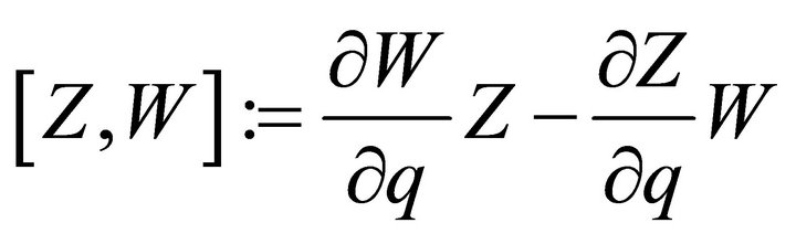
(c) For two vector fields,

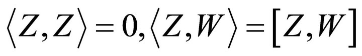(11)

holds.

It is the main characteristic for the rheonomous bracket that the rheonomous affine vector field is perceived as special, and this yields an additional term of a time differential of a vector field as the property (b). It must be also noted that from Definition 2 the rheonomous bracket is equivalent to the normal Lie bracket for scleronomous affine constraints, that is, constraints that do not contain the time variable explicitly. From the next proposition, it turns out that the rheonomous bracket has some important characteristics in common with the Lie bracket.

Proposition 1

For the vector fields on the geometric representation of the fully rheonomous affine constraints (2): and the set of iterated vector fields of them:, the following properties (a), (b), and (c) hold.

(a) Bilinearlity:

(12)

(b) Skew-symmetry:

(13)

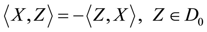
(c) Jacobi’s identity:

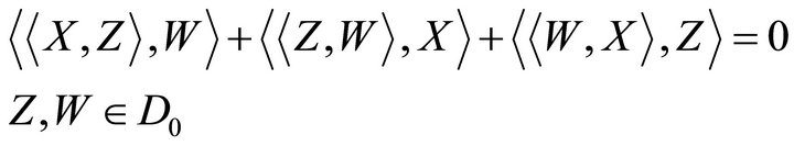(14)

(Proof)

Based on the definition of the rheonomous bracket, we can calculate as follows:

Hence, we complete the proof of (a). Next, a simple calculation can show

Therefore, (b) holds. Finally, we shall prove (c). Since we can calculate the following:

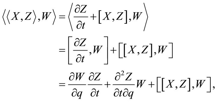
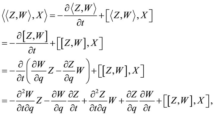
we then obtain

where we utilize Jacobi’s identity for the normal Lie bracket. Consequently, the proof of (c) is completed.

From the properties in Proposition 1, it turns out that we only have to consider the iterated rheonomous brackets in the form:

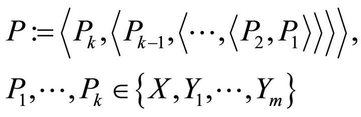(15)

in checking a complete integrability condition for the fully rheonomous affine constraints, which will be shown in the next section. Furthermore, the Philip Hall basis [14], which is a systematic method to generate iterated Lie brackets with an order efficiently, can be also constructed for the rheonomous bracket as follows.

Algorithm 1

For iterated rheonomous brackets (15) of the geometric representation of the fully rheonomous affine constraints (2):, we define the length of (15) as, that is, the number of vector fields in the iterated rheonomous bracket. In addition, the symbol means the magnitude relation for two iterated rheonomous brackets. Then, the Philip Hall basis for the rheonomous bracket can be constructed by the next rules.

(a) are the first elements of and.

(b) If, then.

(c) if and only if and

, either or holds or with and.

4. Complete Integrability Condition

After that, this section investigates complete integrability for the fully rheonomous affine constraints (2). If all the $n − m$ rheonomous affine constraints (2) are integrable, that is, there exist $n − m$ independent first integrals of (2), then they are said to be completely integrable. Now, we define a smallest and involutive time-varying distribution that contains and iterated rheonomous brackets of them, and satisfies

, that is, is spanned by all the rheonomous brackets of with the exception of. Then, we can derive a necessary and sufficient condition on complete integrability for the fully rheonomous affine constraints (2) as the next theorem.

Theorem 1

For the fully rheonomous affine constraints defined on an $n$-dimensional manifold (2) and a time interval, the following statements (a) and (b) are equivalent to each other. If they hold, the fully rheonomous affine constraints (2) are said to be completely integrable.

(a) There exist independent first integrals of the fully rheonomous affine constraints (2).

(b) For a smallest and involutive time-varying distribution,

(16)

holds.

(Proof)

Let us consider the -dimensional product space, where is the space of the time variable, and the local coordinate of is given by

. On, the fully rheonomous affine constraints (2) can be represented by Pfaffian equations of differential forms:

(17)

Since the rheonomous affine vector field of geometric representation satisfies (7), vector fields on which annihilate (17) are given by

(18)

We now define an involutive distribution defined on which contains and iterated Lie brackets that consist of. Therefore, from Frobenius’ theorem [11-14], we can see that a necessary and sufficient condition on complete integrability for (17) is given by

. (19)

Calculating the iterated Lie brackets which consist of, then we have

(20)

It turns out that is independent of and the iterated Lie brackets (20). Hence, we can change the necessary and sufficient condition (19) into the condition such that and the iterated Lie brackets which consist of span an -dimensional space. From (18) and (20), we only have to consider on instead of on, and iterated rheonomous brackets which consist of on instead of Lie brackets which consist of on. Consequently, a necessary and sufficient condition on complete nonholonomicity for the fully rheonomous affine constraints (2) is that and the iterated rheonomous brackets which consist of span an -dimensional space, that is, (16) holds.

From the result of Theorem 1, it can be confirmed that the complete integrability condition for the fully rheonomous affine constraints (2) is quite simple and has a similar structure as the ones for the scleronomous affine constraints and the A-rheonomous affine constraints [6,7], Moreover, we can see that the rheonomous bracket plays a significant role in the condition (16).

5. Example

Finally, in this section, we shall deal with an example in order to evaluate our new results. We consider a 3-dimensional configuration manifold:

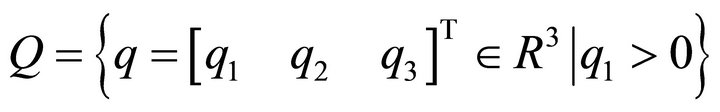(21)

with, and a fully rheonomous affine constraints on:

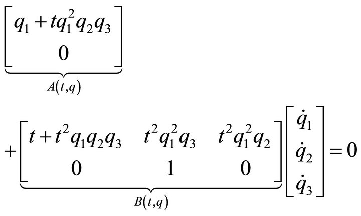(22)

with. We here consider a time interval. It can be confirmed that Assumption 1 holds for (22). One geometric representation for (22) can be obtained as follows:

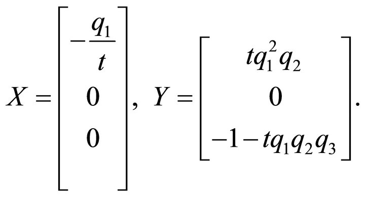(23)

Calculating an iterated rheonomous bracket for and above, we obtain

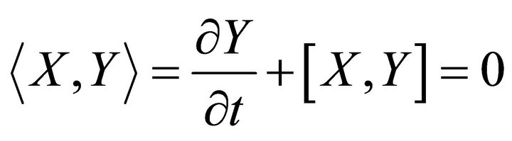. (24)

Hence, we can see that all the iterated rheonomous brackets for are 0. Therefore, we have

(25)

and then it turns out that

(26)

holds.

From Theorem 1, it is confirmed that the fully rheonomous affine constraints (22) are completely integrable.

In fact, there exist two independent first integrals of (22):

(27)

where is the initial point at the initial time.

6. Conclusions

In this paper, we have derived some important properties of the rheonomous bracket and developed a necessary and sufficient condition on complete integrability for the fully rheonomous affine constraints, which is an extension of Frobenius’ theorem for the linear constraints. We can say that the condition is easy to utilize because of its simple structure due to the rheonomous bracket, and the results obtained in this paper provide a fundamental mathematical tool for analysis of systems subject to rheonomous affine constraints.

Future work in this research theme includes development of integrating algorithm for the fully rheonomous affine constraints, applications to control of systems subject to the fully rheonomous affine constraints, and extensions to more general classes of constraints.

7. Acknowledgement

This work was supported by JSPS KAKENHI Grant Number 24760339.

REFERENCES

- J. Cortes, “Geometric, Control and Numerical Aspects of Nonholonomic Systems,” Springer-Verlag, Berlin, Heidelberg, 2002. doi:10.1007/b84020
- A. M. Bloch, “Nonholonomic Mechanics and Control,” Springer-Verlag, New York, 2003. doi:10.1007/b97376
- F. Bullo and A. D. Rewis, “Geometric Control of Mechanical Systems,” Springer-Verlag, New York, 2004.
- R. Montgomery, “A Tour of Subriemannian Geometries, Their Geodesics and Applications,” American Mathematical Society, 2002.
- O. Calin and D. C. Change, “Sub-Riemannian Geometry: General Theory and Examples,” Cambridge University Press, Cambridge, 2009. doi:10.1017/CBO9781139195966
- T. Kai and H. Kimura, “Theoretical Analysis of Affine Constraints on a Configuration Manifold—Part I: Integrability and Nonintegrability Conditions for Affine Constraints and Foliation Structures of a Configuration Manifold,” Transactions of the Society of Instrument and Control Engineers, Vol. 42, No. 3, 2006, pp. 212-221.
- T. Kai, “Integrating Algorithms for Integrable Affine Constraints,” IEICE Transactions on Fundamentals of Electronics, Communications and Computer Sciences, Vol. E94-A, No. 1, 2011, pp. 464-467.
- T. Kai, “Mathematical Modelling and Theoretical Analysis of Nonholonomic Kinematic Systems with a Class of Rheonomous Affine Constraints,” Applied Mathematical Modelling, Vol. 36, No. 7, 2012, pp. 3189-3200. doi:10.1016/j.apm.2011.10.015
- T. Kai, “Theoretical Analysis for a Class of Rheonomous Affine Constraints on Configuration Manifolds—Part I: Fundamental Properties and Integrability/Nonintegrability Conditions,” Mathematical Problems in Engineering, Vol. 2012, 2012, Article ID: 543098. doi:10.1155/2012/543098
- T. Kai, “Theoretical Analysis for a Class of Rheonomous Affine Constraints on Configuration Manifolds—Part II: Foliation Structures and Integrating Algorithms,” Mathematical Problems in Engineering, Vol. 2012, 2012, Article ID: 345942. doi:10.1155/2012/345942
- S. Nomizu and K. Kobayashi, “Foundations of Differential Geometry Volume I,” John Wiley & Sons Inc., New York, 1996.
- S. Nomizu and K. Kobayashi, “Foundations of Differential Geometry Volume II,” John Wiley & Sons Inc., New York, 1996.
- A. Isidori, “Nonlinear Control Systems,” 3rd Edition, Springer-Verlag, London, 1995. doi:10.1007/978-1-84628-615-5
- S. S. Sastry, “Nonlinear Systems,” Springer-Verlag, New York, 1999. doi:10.1007/978-1-4757-3108-8