Open Journal of Fluid Dynamics
Vol.07 No.03(2017), Article ID:79057,22 pages
10.4236/ojfd.2017.73019
Simulating Spiraling Bubble Movement in the EL Approach
Andreas Weber1, Hans-Jörg Bart1, Axel Klar2
1Department of Separation Science and Technology, TU Kaiserslautern, Kaiserslautern, Germany
2Department of Technomathematics, TU Kaiserslautern, Kaiserslautern, Germany

Copyright © 2017 by authors and Scientific Research Publishing Inc.
This work is licensed under the Creative Commons Attribution International License (CC BY 4.0).
http://creativecommons.org/licenses/by/4.0/


Received: August 10, 2017; Accepted: September 11, 2017; Published: September 14, 2017
ABSTRACT
Simulating the detailed movement of a rising bubble can be challenging, especially when it comes to bubble path instabilities. A solution based on the Euler Lagrange (EL) approach is presented, where the bubbles show oscillating shape and/or instable paths while computational cost are at a far lower level than in DNS. The model calculates direction, shape and rotation of the bubbles. A lateral force based on rotation and direction is modeled to finally create typical instable path lines. This is embedded in an EL simulation, which can resolve bubble size distribution, mass transfer and chemical reactions. A parameter study was used to choose appropriate model constants for a mean bubble size of 3 mm. To ensure realistic solution, validation against experimental data of single rising bubbles and bubble swarms are presented. References with 2D and also 3D analysis are taken into account to compare simulative data in terms of typical geometrical parameters and average field values.
Keywords:
Euler Lagrange, Bubble Column, Bubble Path Instability, Ellipsoidal Bubble, Bubble Shape, Zigzag Path

1. Introduction
Understanding bubbles path instabilities during rise in bubble columns is a major challenge since the 1960s. Early measurements were performed by [1] , where a single bubble was rising in a fluid showing different path lines, like zigzag and spiraling. Nowadays, a 3D camera setup enables a more detailed view [2] and sophisticated simulations [3] could help to explain the complex rising behavior. The origin of this behavior is in the turbulent eddies induced behind the bubble during its rise. Instabilities in these eddies lead to an eccentric force on the bubble, which then leads to a deviation from a straight rise resulting into a spiraling or zigzagging path. The development of the turbulent eddy behind a bubble is connected also to its shape and size. Different types of bubble paths can be experienced, based on the bubble size or, in terms of turbulence intensity, on the bubble Reynolds number.
Simulating bubble hydrodynamics is an issue since many years ago. The most common approach to do this is the simplified Euler Euler (EE) method, where single bubbles are no longer resolved but a bubble number density is taken into account instead. Bubbles located in a computational cell are supposed to have identical velocity and bubble sizes are often reduced to characteristic mean values (d32, d10) for the calculation. Interaction of bubbles is no longer a problem, since simple source terms can be used to simulate changes in the bubble size distribution. This also leads to a much simpler way to calculate for an instable bubble path, namely a diffusion term is used. This gives a high loss of detail on the bubble scale while the overall spatial distribution of bubbles can be forecast with adequate precision.
The other extreme is a high detail direct numerical simulation (DNS) of a single bubble or rather a small bubble swarm. Bubbles are resolved in full detail including the interfacial area deformations and the hydrodynamics inside. Turbulence in- and outside the bubbles are also calculated in high detail, trailing eddies in the bubble wake flow are resolved. In doing so, path instabilities can be simulated consequently on the lowest level of scale but at a high computational load. The DNS is unsuitable for simulation of a whole bubble column reactor because of its sheer bubble number. Despite the detailed flow simulation of the single bubble, the DNS is not capable of simulating a reliable behavior when bubbles coalesce or breakage happens. Those processes take place on an even lower spatial scale at the bubble surface layer and need special modeling, e.g. sub-grid models [4] .
Free rising ellipsoidal bubbles not only move in straight lines but can describe sinusoidal, zigzag or spiraling paths. The common Euler Euler (EE) simulation techniques can no longer resolve the actual movement patterns and Direct Numerical Simulations (DNS) tend to be very costly when simulating a larger number of bubbles. This work presents a solution to calculate the orientation and shape of bubbles using the Euler Lagrange (EL) approach. Advantages lie within the fast computation and the high level of detail. In comparison to DNS, the insides of the bubbles are not calculated in full detail but macroscopic models are employed. Every bubble is calculated individually, having its own size, direction and shape. The surrounding fluid will influence not only the bubble’s movement but also the rotation and shape. The actual calculation of the turbulent eddies behind the bubble will not be carried out, but an oscillation orientation model is used and model parameters are calibrated from experimental data. This enables the simulation of instable bubble paths, while the bubble number can easily exceed those of a DNS simulation. The EL approach is also capable of evaluating the bubble size distribution due to coalescence and break-up by stochastic modeling. The individual simulation of each bubble allows more detailed simulation of bubble dynamics, e.g. mass transfer or residence time characteristics, than it is possible in the EE approach. With the implemented shape factor estimation, physical models could be expanded to account for the deformed bubble surface area.
2. EL Modeling
The general EL model describes bubbles as a point volume acting under Newtonian dynamics. Forces created by the surrounding fluid and neighboring bubbles accelerate these Lagrangian points through the domain. The continuous phase itself is calculated using Navier-Stokes equations and can be coupled to the interaction forces by a source term. All forces are calculated for each bubble individually, which produces an individual path for each bubble. Therein lies one of the advantage of the EL approach in comparison to the EE methods. Bubbles can coalesce and break, which gives a bubble size distribution, with even more detail than common method of moments approaches. Downside of the EL approach is the higher computational load, which is strongly dependent on the number of bubbles simulated. Nevertheless, the EL approach has been used frequently in several different simulations of bubbly flow [5] .
2.1. Liquid Phase Hydrodynamics
The continuous phase is assumed to be incompressible, basis for calculation is a modified Navier-Stokes equation:
(1)
Given is the continuous velocity uc, the pressure p, the density ρ, the viscosity μ and the source term f. The source term f depicts the forces of the bubbles and will thereby serve as a coupling of the phases. Turbulence is computed using the standard RANS k-epsilon model [6] with additional bubble induce turbulence (BIT) [7] . Each bubbles’ drag force induces turbulent energy and dissipation in the associated computational grid cell. For each cell this sums up and is added to the source term in the turbulence model.
(2)
(3)
(4)
Here, Sk denotes the source term for the turbulent energy k, FD stands for the drag force. Sε is the turbulent dissipation with τ, the turbulent time scale.
2.2. Bubble Hydrodynamics
Bubbles are modeled as point volumes acting under Newtonian dynamics. Their movement is calculated using a number of different forces.
(5)
The sum of forces consists of the buoyancy and weight force FB, the drag force FD, the lift force FL, the virtual mass force FVM, the wall lubrication force FW and the bubble dispersion force FBD. Here the subscripts b and c stand for the bubble and the continuous phase accordingly, the subscript rel identifies the relative differences between them. Furthermore, g denotes the gravitational acceleration, ρ stands for densities, u for velocity, V for the bubble’s volume, k for the turbulent kinetic energy and α for the phase fraction. Appropriate model parameters are denoted with Ci.
(6)
(7)
(8)
(9)
(10)
(11)
Di/Dt in Equation (9) denotes the material derivative, meaning that the derivative is made while following the bubble. Drag and lift force coefficients CD, CL are calculated using the models of [8] . The virtual mass coefficient is set to CVM = 0.5 according to [9] , the coefficient for the dispersion force is set to CTD = 0.1 [10] . This dispersion describes the ambition of bubbles to spread due to collisions with other bubbles. Additionally, a second turbulent dispersion is used to model the collision of bubbles and turbulent eddies. The Random Dispersion Model [11] is used to calculate eddies according to the surrounding level of turbulence. Assuming an isotropic turbulence, eddies are traveling through the liquid in a uniformly random direction with a specific life time. In the model, the turbulent eddy lifetime tE is evaluated, after which a new eddy is calculated.
(12)
Then the movement direction of the eddy is uniformly chosen while its velocity follows a normal distribution with a variance dependent on the turbulent energy k.
(13)
This turbulent velocity is added to the underlying continuous phase velocity for each bubble individually, which is then used to calculate the different bubble forces. Especially the drag force calculation is a crucial step to produce dispersion of the bubbles. In order to achieve the same amount of bubble dispersion like in the experiment, the turbulent velocity for drag force calculation had to be slightly increased.
Change in bubble volume due to the pressure drop while rising is calculated assuming an ideal gas. Mass transfer and/or chemical reactions are not considered in this simulation.
2.3. Ellipsoidal Bubble Model
According to the state of the art of bubble simulations almost any model assumptions are based on bubbles having a spherical shape. Simplest example is the Sauter diameter d32, which maps the mean volume/surface area ratio of a bubble population to one spherical bubble size. Collision frequency or rather probability, e.g. by [12] , is based on the calculation of the overlapping volume of spheres. Other examples are mass transfer calculation (spherical transport area), coalescence and break-up (interfacial energy of spheres) or simply the distance calculation between bubbles or wall and bubble. Only exception is the drag force, which is often modeled with respect to the shape of the bubble e.g. by [8] but uses no information about orientation or rotation of the bubble. One has to admit, that the assumption of bubbles being spheres is adequate for many problems. For example, the deviation of the collision probability is negligible if a spatially uniform random orientation of the bubbles is assumed. Nevertheless, for the computation of realistic bubble movement, a better model for the bubble shape has to be chosen.
In this work, the deformed bubble will be approximated with an oblate spheroid, an ellipsoid with two different axes a and c, where c > a. For simplicities sake, all following figures will contain a simplified 2D version of the spheroid in Figure 1.
The ratio of the axes is chosen to describe the bubble shape via the shape factor sf.
(14)

Figure 1. An oblate spheroid.
A shape factor of sf = 1 describes a perfect spherical shape, while a lower value stands for a more deformed sphere and sf = 0 would describe an infinitely thinned spheroid. Some models are based on empirical measurements using dimensionless numbers for the calculation, others are physical models derived from the interfacial tension and pressure distribution. It turned out that a good result for the simulation problem was achieved by [13] with the underlying equation:
(15)
Since the shape factor has to be computed as a function of the Weber number, an approximation has been used:
(16)
Note that this equation is based on the dimensionless Weber number, which can represent changes in the shape induced by fluctuating relative velocities. The critical Weber Number Wecrit = 3.745 describes the transition to irregular bubble shapes. If the current Weber number is higher than Wecrit a shape factor of sf = 0.2 is chosen.
(17)
Implementing the new bubble shape into the CFD framework necessitates further usage of the diameter definition of a spherical bubble. The volume of the sphere should be equal to the oblate spheroid volume, which leads to the following basic equations:
(18)
(19)
(20)
Differently than with common rotation calculation, using the moment of inertia and torque action [14] , an approach originally developed by [15] is used. The direction of the bubble is described by a vector p pointing in the direction of axis a. The change in direction is given as the vector , which is deduced from the rotation vector ω (s. Figure 2). This notation is beneficial because there is no need for a change to spherical coordinates (Θ, Φ), which would lead to higher computational load. The only requirement is a sufficiently small change of the vector p, which is fulfilled within the computed time step of the simulation.
(21)
This rotation notation has been used by [16] to calculate the orientation of
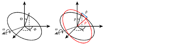
Figure 2. Left: orientation in spherical coordinates; right: orientation with vectors p and .
rigid ellipsoidal bodies in a Stokes flow. Based on these equations, a modified model for ellipsoidal bubbles was developed. In general, the bubble rotation is calculated using an explicit Euler algorithm:
(22)
(23)
Just as the bubble’s position and velocity, the orientation p changes due to the orientation change . The bubble’s rotation relaxes against the outer rotation G with the factor . Here, denotes a simplified interaction of the bubble’s moment of inertia and torque. A low implies a high bubble mass/inertia and thus a slower rotation due to outer forces. The additional term resembles a random rotation due to turbulence, where is used to scale the effect of turbulent randomness. It is generated similarly to the turbulent dispersion velocity . Since the effective moment of inertia of a gas bubble inside a fluid is unknown, has to be derived from experimental data.
(24)
(25)
The outer rotation G is a summation of three main mechanics acting on the body Equation (24). The first line implies that the rotation of the surrounding fluid is transmitted to the bubble itself. The second line describes the rotation induced by shear stress in the surrounding fluid, S[uC] is the symmetric part of the Jacobian matrix.
(26)
The third line is an addition to the original model [16] and describes the ambition of the gas bubble to orient itself along the gravitation direction g. Since the original equation was deduced for rigid bodies only, all of the above-mentioned mechanics are weighted by the parameters Ji to fit experimental data of (non-rigid) bubbles. This also compensates for the fact, that there is no Stokes flow around the bubble and its interface is mobile (slip condition).
Especially the third line of Equation (24) leads to an oscillatory system, which enables the bubble to describe sinusoidal or helical orientation characteristics. While the orientation of the bubble is changing, the vector of orientation change will eventually point to a direction not perpendicular to p, thus rising in size and finally damping and stopping the oscillation. To prevent this, the direction change vector will be moved to the plane normal to the orientation vector by subtracting the part parallel to it:
(27)
In total, this will lead to a slight damping of the oscillation, which can be eliminated by preserving the magnitude of the orientation change vector:
(28)
To preserve robust behavior a slight damping (δ = 0.2) is executed for the orientation change:
(29)
Finally, with an interaction force based on the orientation, the bubble experiences a drift perpendicular to the main movement direction. This results in a bubble trajectory describing helical and sinusoidal (zigzag) paths. This perpendicular force has the same direction as the change in direction [3] , which gives (Figure 3):
(30)

Figure 3. Direction of forces and direction change on a sinusoidal bubble path.
This force is modeled as a modified drag force. Also, to imitate real bubble behavior, we limit the force to only occur on bubbles within a certain range of Reynolds number [1] . This will stop the oscillating motion for very small (d < 0.8 mm) and large bubbles (d > 3.5 mm) as observed in experiments.
(31)
The additional side force due to bubble rotation is modeled with the magnitude of the current drag force FD and the bubble rotation but will point in the direction of rotation. It turned out, that a scaling linear to the magnitude of the direction change will lead to instabilities easily, which can be stabilized by using the square root instead. The bubble path amplitude is calibrated with the parameter β, where a higher value implies a larger amplitude of the resulting oscillating path.
3. Parameter Estimation
Parameters , R and Ji (Equations (22) and (23)) are derived from a parameter study and with analysis of the oscillatory equations. The characteristic bubble path amplitudes, frequency and wavelength shown in [2] were taken to set first limits to the parameter study. In a more detailed analysis, the parameters are correlated to experimental data showing bubble swarms rather than single rising bubbles. The resulting simulated bubble paths are then compared to experimental data from the Bubble Column Reactor Database of the University of Magdeburg (http://www.uni-magdeburg.de/isut/LSS/spp1740/). Characteristic oscillatory dimensions can be derived from Equation (23) and the third line of Equation (24). This will lead to a simple harmonic oscillator equation with the following form:
(32)
with
(33)
Without damping of the oscillation, the frequency f0 can be calculated with the parameters J3 and .
(34)
It turned out, that this is the case for our oscillatory system, but only if the random rotation is set to zero. A case without random rotation was set up for this reason, the results are shown in Figure 4. Over a wide range, the simulated frequency is identical to the analytical solution for the undamped oscillation.
Most references are made on a basis of a stagnant liquid phase, such that the bubble rise velocity ub can be easily estimated. This makes it easy to calculate an appropriate wavelength of the generated/observed bubble path using its characteristic

Figure 4. Oscillation parameters vs. bubble path frequency.
frequency.
(35)
In case of a non-stagnant liquid, like in a bubble column, the bubble velocity has to be identified at first. It is therefore important to mention, that the wavelength of a bubble path in a dynamic system will differ from most reference experiments, which are made using a well-defined surrounding. Also, in some areas of the column a downward flow occurs, lowering the bubble’s rising velocity. To overcome this problem, the bubble velocity and/or wavelengths are averaged over a large number of bubble paths.
3.1. Experimental Setup
For the parameter study, simulation results were compared to experimental measurements from the Institut für Strömungstechnik und Thermodynamik, University of Magdeburg [17] [18] [19] . The experimental setup consists of a cylindrical air-water bubble column with an inner diameter of 14.22 cm and a filling height of 73 cm. The air inlets are positioned at the bottom of the column and consist of four nozzles in a row. The distance between nozzles is 2.2 cm. The measurements were made with a camera system facing the four nozzles side by side (front view) and were also done a second time when facing the nozzles behind each other (side view). A high-resolution camera and a backlight system produce shadow graphic images of the bubbles, which have been processed to gain information about bubble size, shape and velocity. With a frame rate of 100 Hz the position of a bubble shows only little change in consecutive picture. This enables tracking of a bubble by searching for the closest position in the subsequent picture (Figure 5). With this method, the bubble positions and velocities were captured and the trajectories have been reconstructed. With an air throughput of 10 l/h a mean bubble size of d = 3 mm was measured using the same camera setup.
An automated analysis was used to estimate the characteristic path shapes,

Figure 5. Schematic experimental setup: 1: Camera; 2: Light source; 3: Diffused backlight; 4: Bubble column.
given by the mean and standard deviation of the wavelength and amplitude A of all bubble paths. To ensure a correct analysis, only those trajectories were considered, that were of appropriate length (minimum of 30 measured positions). Unfortunately, a 3D reconstruction was not possible for the bubble paths, because the side view measurements were not made simultaneously with the front view.
In addition, the liquid velocity was measured using Particle Image Velocimetry (PIV). Small tracer particles were added to the fluid and illuminated by a laser light sheet. This laser projection grants insight to the cross-sectional liquid velocity inside the column.
3.2. Computational Setup
The corresponding computational mesh was created using a rectangular grid of 28 × 28 × 146 cells with overlapping cells being removed and reshaped to fit the cylindrical shape. This results in a mesh with 90,000 cells, shown in Figure 6. Mesh resolution was intentionally left at approximately 0.125 cm3 per cell (mean cell length of 0.5 cm), because the bubble size must be smaller than the cell size in our EL approach. Cells near the walls are not rectangular anymore, but are also solemnly populated by bubbles due to wall lubrication force. The main bubble flow therefore happens in the center part, where the cells are in perfect rectangular shape.
For boundary conditions (s. Table 1), the simplest possible case could be adopted. All walls except the top outlet patch are combined and have the same properties. Since bubbles are injected using the Lagrangian approach, there is no need for an inlet patch. Instead of a free surface at the top, a slip condition has been set. This approach enables to use a single phase solver but is surely not

Figure 6. Computational mesh of the cylindrical bubble column.

Table 1. Boundary conditions.
suitable for estimating hydrodynamics near the surface. Since our interest lies within the lower part of the column, this error is acceptable.
On the basis of the experimental measurements, the mean inlet diameter of the bubbles was set to d = 3 mm. With a throughput of 10 l/h this leads to a total number of 196.4 bubbles per second to inject from the four nozzles. Bubble breakup, coalescence and mass transfer was turned off in this case, since only the bubble movement is of concern and measurements showed only a minimum of bubble size variations during rise. The experimental measurement area is positioned in the lower 312 mm of the column only, but the whole height of the column was simulated to achieve the correct flow pattern.
Since there are 4 parameters in total to be calibrated, an automated parameter study software has been used (Dakota, Sandia National Laboratories) to simulate a variety of combinations. The target function was the characteristic bubble flow path parameters, which were compared by screenshots at a first sight. After choosing the most promising parameter interval, a detailed analysis of bubble path frequency and amplitude followed. Therefore, an automated analysis of the generated path lines was used to calculate for mean wavelength and amplitude (~600 trajectories per simulation). The same method has been used to characterize the experimental measurements. Since the experimental data was collected using a 2D visual acquisition, simulation results were also calculated using a 2D mapping. Additionally, a 3D analysis was made and compared to other reference measurements.
4. Results and Discussion
4.1. Velocity Profiles
Simulated liquid velocity and its deviation are compared to the experimental measurements by the Institut für Strömungstechnik und Thermodynamik, University of Magdeburg in Figure 7. The upper figure shows the mean vertical velocity of experiment (left) and simulation (right) on the middle plane of the

Figure 7. Mean vertical velocity. Upper figure: overview (left: experiment, right: simulation), (A)-(D) depicts the detailed line plot positions. (A)-(D): detailed line plots on different heights.
column. The white line represents the zero value, making it easier to spot the upward and downward flow area. The scale depicted on the left side shows the detailed line plot positions (A)-(D) in the lower figures. The liquid velocity profile from the experimental measurements shows a slower flow than the simulation produced. Probable reason for this could lie within the modifications done to the drag force calculations in order to acquire the special bubble movement. It has not yet been optimized in order to sustain an appropriate liquid velocity. Also, the liquid phase resolution is quite low in order to maintain an appropriate aspect ratio of bubble length to cell length. Aim of this work lies within the simulation of correct bubble paths rather than optimal liquid phase hydrodynamics.
Calculation of the simulated fluctuating velocity is made using the k-epsilon turbulence model. Values described here (s. Figure 8) are solution of the turbulent energy k with assumed isotropic turbulence velocities:
(36)
The upper figure shows the fluctuating velocity deviation of the experiment by the Institut für Strömungstechnik und Thermodynamik, University of Magdeburg (left) and simulation (right) on the middle plane of the column. Again, the scale on the left side shows the line plot positions A-D. In the lower sections, the fluctuation velocity is similar to the measured values from the experiments. In higher sections, the simulation underestimates the level of turbulence, leading to low fluctuating velocities in comparison to experimental data. Here again, a standard parameter set was used for the BIT model [20] . It was not optimized on this particular case as investigations on bubble induced turbulence was also not in the focus. However, as a consequence the impact of turbulence on bubble rotation is adjusted via the parameter study.
4.2. Bubble Path Characteristics
According to literature [14] , the bubble path oscillations of a single air bubble (d = 3 mm) rising in tap water is approximately f0 = 5 s−1. With its mean free rising velocity of ub = 35 cm/s the bubble path wavelength is λ = 7 cm. According to Equation (34) this would recommend setting the parameter .
Anyhow, analysis of the experimental data from the University of Magdeburg yielded a mean bubble path wavelength of λ = 4.14 cm and an amplitude of A = 1.87 mm. Mean bubble rise velocity is ub = 29 cm/s in this case which gives a frequency of f0 = 7 s−1 and a product of parameters of . This was only a first estimation, since the random rotation has not been set to zero in the final simulation.
Experimental data from 4 different measurements on the same properties were used to reconstruct and analyze bubble trajectories (s. Table 2). The trailing numbers in the Case name stand for the frame rate and the number of frames used in the analysis. A given frame rate of 0.1 kHz and 100, 250 or 500

Figure 8. Standard deviation of velocity fluctuations. Upper figure: overview (left: experiment, right: simulation), (A)-(D) depicts the detailed line plot positions. (A)-(D): detailed line plots on different heights.
frames implies a measuring time of 1, 2.5 or 5 seconds accordingly. In order to estimate characteristic trajectory wavelengths and amplitudes, the points of inflexion of each trajectory were determined. Since main movement direction is upwards, the inflexion point distance in vertical direction was used to identify the wavelength while the horizontal distance was used for the amplitude. Averaging over all trajectories yields the characteristic wavelength and amplitude with their deviations. This method was used for both, the experimental and the
Table 2. Characteristic path lengths (all values in mm).
simulative data. Deviation of wavelength and especially of amplitude is quite high, which is partly owed to the 2D analysis of the bubble paths. Since a flat zigzag path can only be seen correctly from one perspective, the calculated 2D amplitude will hardly correspond to the true 3D amplitude, it will generally underestimate the true value. This is why the standard deviation of the analyzed amplitude show rather high values in all experimental and simulation cases.
With the appropriate set of parameters, the simulated bubble path characteristics properly match the experimental values (Table 3). Final simulations show that the assumed parameter to 2000 is a quite good starting value, the most promising results were done with parameters in the range of to 1350. It turned out that the values of the parameters for direct influence of liquid rotation (γJ1) and shear (γJ2) are very low in contrast to the oscillation (γJ3), while the random factor (R) is of the same magnitude. Thus, the impact of rotational/shear flow around bubbles plays a minor role on the rotation while it is dictated mostly by turbulent eddies hitting the bubbles.
A visual comparison of the three most promising bubble paths in Figure 9 reveal only few evident differences. The overall shape and distribution of path lines is almost identical. Most noticeable differences can be observed directly at the bubble inlets at the very bottom of the column. In the simulation, bubbles are spread earlier than it is observed in the experiments. In the experiment, bubbles describe a straight line directly after being injected to the column, while the simulation shows a rotation of the bubbles at the very beginning of the path, pushing the bubbles into a turn after the injection. In the first 100 mm, a pattern can be seen in the flow paths of the simulation. The flow in the middle of the column pushes the bubbles away from the middle line, creating an area where almost no bubble cross. Some bubbles tend to take the same path multiple times, while in the experiment a slightly more chaotic distribution is present. In the
Table 3. Parameter sets for the three most promising simulations.
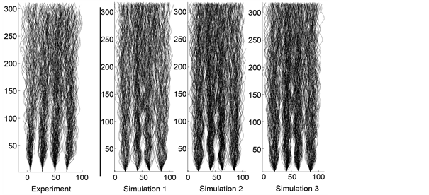
Figure 9. Reconstructed bubble trajectories, axes in mm. Left: experimental results; right: simulation results.
simulation, a parameter for random rotation is used, but the analysis does not concern the overall distribution of bubbles. The spread/diffusion of bubbles in the upper area however (height > 150 mm) yields no (qualitatively) visible difference between experiment and simulation.
Another point of concern is the behavior of the simulated orientation in comparison with the velocity of the bubble. In order to describe this relations, different deduced angles are used; the movement angle lies between the vertical axis (gravitational direction) and movement direction, the orientation angle is between the short axis direction and vertical axis and the drift angle lies between orientation and movement vectors. With 2D analysis of the simulation data, the orientation angles show a normal distribution with mean value near to zero (Figure 10, left), just like the experimental results [21] . A 3D analysis however proves the oversimplification when using 2D analysis because the simulated mean 3D orientation is 18.3˚. This gets clear when figuring a perfectly spiraling path seen from only one side, where there is a constant orientation angle in reality but an alternating angle is seen from a fixed observer. In a worst case scenario, a flat sinusoidal path oscillates parallel to the line of sight, thus making it impossible to see any oscillations at all.
Bubble velocity and orientation vectors roughly point to the same direction, this has been shown in several references [3] [21] [22] , which implies a small drift angle. Simulation results also show mostly small drift angles (Figure 10,
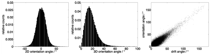
Figure 10. Characteristic angles between velocity and orientation vectors of simulated bubbles. Left: orientation angle using 2D data; middle: orientation angle using 3D data; right: drift angle vs. orientation angle (3D data).
right) with a mean value of 19.2˚. Experimental data shows, that the largest drift angles occur at the most outer points of the oscillation, especially when a planar zigzag path is fulfilled [3] . This means a high drift occurs when the orientation angle is near zero. Simulation data shows other characteristics; a high drift angle correlates with a high orientation angle (s. Figure 10, right). In DNS simulation, the drift and orientation angles have shown sinusoidal characteristics, while both were 90˚ out of phase. In the EL simulation these angles are in phase. Unfortunately, there is no experimental proof for this correlation with 3D measurements in a bubble swarm.
When taking a closer look at single trajectories of one of the bubbles rising in the swarm it will reveal characteristic parts of the bubble’s movement. As shown in [22] , the bubble paths can be described as “flattened helixes” which become less flattened while rising. Exactly this behavior can be found in the simulated bubble paths depicted in Figure 11. The bubble path shown here is not picked randomly, since characteristic movement is not achieved with every bubble. Note that this simulation considers bubbles in a large swarm rather than single rising bubbles (like in the experimental reference). This leads to a more chaotic liquid and bubble movement, which can abruptly change bubble movement direction and orientation. Near the walls, a downward flow occurs in which bubbles performed differently, mostly not showing steady oscillations. As most bubbles rising in the middle part of the column, oscillation slowly starts within the lower 100 mm where it evolves to a sinusoidal and finally to a helical path (at approx. 400 mm height).
We can observe influence of the flow in terms of a strong drift in the bubble paths (s. Figure 11, top row). In order to give a three dimensional description of the paths, a polynomial fit (n = 3) is used to smooth out the bubbles drift movement. In Figure 11 (top row) the original bubble paths are shown from three sides with the polynomial fit (dotted line). The bubble paths are normalized using the polynomial fit and the resulting path data (s. Figure 11, bottom row) describes a spiral, which is more comparable to experimental work (where the drift movement is almost zero). Assuming that our path describes a perfect flattened spiral, its coordinates perpendicular to the rising direction can be taken to
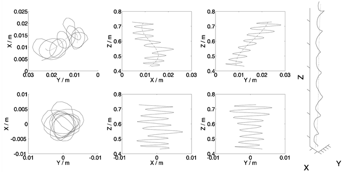
Figure 11. Single bubble trajectory. Top row: raw data with fitted polynomials (dotted lines); bottom row: drift-corrected path data; right: isometric view of the raw path with fitted polynomials (dotted line).
calculate for a “dynamic radius” of the path. A flattened spiral would look like an ellipsoid in the X-Y view (s. Figure 11, bottom left). The maximum of this radius will give the amplitude of the major oscillation mode, while the minimum will give the minor modes amplitude. When the minor amplitude is zero, a completely flat spiral, a planar zigzag path, is present. In addition, the wavelength in rising direction can be extracted from this data by measuring the distance for one spiral rotation. Due to measurement errors with 2D data, a larger amplitude can be expected in 3D analysis. In Simulation case 1 the mean (3D) wavelength is λ = 4.79 cm and mean amplitude is A = 4.04 mm. This is a much larger amplitude, than it has been calculated for the 2D analysis, but comparison with [22] shows a good match. They analyzed a single rising bubble with equivalent diameter d = 2.48 mm and could measure a major mode amplitude of A = 4.3 mm. Measured path frequency was ω = 39 rad/s, which is ω = 35.4 rad/s in our simulation case (mean rise velocity ub = 0.264 m/s). Oldest related work [23] contains photographic pictures of a rising bubble and drift correction results very similar to Figure 11. A mean orientation angle of 20˚ and a frequency of 6.25 Hz is stated for the rise of a bubble in helical motion. This is in unison with our simulation results, where a mean orientation of 18.3˚ is present and the mean frequency is f = 6.44 Hz. It is also stated that angle and frequency are independent of bubble size, only the path amplitude changes with diameter. This would imply that a simple model could cover a wide range of bubble sizes, by only fitting the appropriate amplitude. A more general overview on instable paths of different bodies is given in [24] . The bubble motion is summarized with amplitudes in the range of 3 - 5 deq, maximum inclination angles from 20˚ to 30˚ and characteristic frequencies in the range of 0.09 < St < 0.15 (St = fL/U = L/λ). In our case, the simulated amplitudes are far lower (~1.5 deq) but inclination angles and frequency are similar (St = 0.073 in our case). Only severe difference is the stated maximum drift angle of only 2˚, which is far higher in our simulation case.
Most deviations to experimental and other simulative work venture from the drift angle characteristics. Since the side force Fs (Equation (31)) is responsible for the horizontal movement, other models should achieve more suitable drift angles. Reference yields only few insights on modeling of this particular force [14] and often parameters are unknown. Furthermore, the parameter fit with 2D data, as in this work, is certainly not suitable for finding an appropriate side force model. Anyway, this simple 2D data fitting technique could still reproduce characteristic bubble trajectories by means of frequency, amplitude and shape.
5. Conclusions
The presented EL simulation is capable of simulating unstable sinusoidal/spiraling bubble paths using macroscopic models. Bubble orientation, rotation and shape are calculated to achieve characteristic movement. Due to the assumption of bubbles describing rotational spheroids, the additional parameters that have to be calculated reduce to a shape factor, rotation and orientation vectors. A force induced by the bubbles rotation produces the lateral force leading to an oscillation movement.
The macroscopic orientation and rotation model uses a simple vector-based approach. The usage of a spherical coordinate system was intentionally rejected to keep the model as simple as possible. The model equations are easy to compute and allow simulating of a large number of bubbles at a time. Unfortunately, only few comparable models exist [14] and performance comparison was not possible. DNS simulations indicate similar results concerning bubble path characteristics but are not comparable in performance issues.
A parameter study was used to fit the model constants to experimental data for mean bubble size of d = 3 mm. Parameter estimation was made using the amplitude and wavelength of the typical spiral movement. It turned out that most 2D measurements cannot reflect characteristic path parameters entirely. Especially, orientation angles are problematic in 2D analysis, because the perspective view only permits seeing angles perpendicular to the line of sight. In order to still achieve a good fit, the simulation results were mapped to a 2D point of view and compared to the experimental data. After parameter fitting, comparison to reference bubble path data was made using 2D and 3D analysis and could prove correct reproduction of unstable bubble paths. Evaluation of the 3D bubble path in a bubble swarm is difficult, since most references only supply 2D camera setups or single bubble trajectories in 3D analysis systems. Comparison to DNS simulation and single rising bubble path data could also show good agreement. Amplitude and wavelength of the simulated bubble path are in unison with the measurements. Detailed comparison of DNS results of the drift angle reveals slight disagreement.
For further improvement of the model, a predictive parameter approach should be used to also cover different bubble sizes. Interaction of deformed bubbles is not considered in the EL model shown here, and this could include collision, break-up, mass transfer and other shape dependent processes.
Acknowledgements
Funding by the Deutsche Forschungsgemeinschaft (DFG) within the RTG GrK 1932 “Stochastic Models for Innovations in the Engineering Sciences”, project area P1, is gratefully acknowledged. We want to thank the Group of K. Zähringer, Laboratory of Fluid Dynamics and Technical Flows, University of Magdeburg, for supplying experimental data on the bubble paths and liquid velocity PIV measurements.
Cite this paper
Weber, A., Bart, H.-J. and Klar, A. (2017) Simulating Spiraling Bubble Movement in the EL Approach. Open Journal of Fluid Dynamics, 7, 288-309. https://doi.org/10.4236/ojfd.2017.73019
References
- 1. Aybers, N.M. and Tapucu, A. (1969) The Motion of Gas Bubbles Rising through Stagnant Liquid. Wärme-und Stoffübertragung, 2, 118-128. https://doi.org/10.1007/BF01089056
- 2. Shew, W.L. and Pinton, J.-F. (2006) Viscoelastic Effects on the Dynamics of a Rising Bubble. Journal of Statistical Mechanics: Theory and Experiment, 01, P01009-P01009. https://doi.org/10.1088/1742-5468/2006/01/P01009
- 3. Mougin, G. and Magnaudet, J. (2006) Wake-Induced Forces and Torques on a Zigzagging/Spralling Bubble. Journal of Fluid Mechanics, 567, 185-194. https://doi.org/10.1017/S0022112006002266
- 4. Mason, L.R., Stevens, G.W. and Harvie, D.J.E. (2012) Multi-Scale Volume of Fluid Modelling of Droplet Coalescence. The 9th International Conference on CFD in the Minerals and Process Industries, Melbourne, 10-12 December 2012, 1-6.
- 5. Gruber, M.C., Radl, S. and Khinast, J.G. (2015) Rigorous Modeling of CO2 Absorption and Chemisorption. The Influence of Bubble Coalescence and Breakage. Chemical Engineering Science, 137, 188-204. https://doi.org/10.1016/j.ces.2015.06.008
- 6. Launder, B.E. and Spalding, D.B. (1972) Lectures in Mathematical Models of Turbulence. Academic Press (London), London, New York.
- 7. Rzehak, R. and Krepper, E. (2013) Bubble-Induced Turbulence: Comparison of CFD Models. Nuclear Engineering and Design, 258, 57-65. https://doi.org/10.1016/j.nucengdes.2013.02.008
- 8. Tomiyama, A. (2004) Drag, Lift and Virtual Mass Force Acting on a Single Bubble. 3rd International Symposium on Two-Phase Flow Modelling and Experimentation, Pisa, 22-25 September 2004, 22-24.
- 9. Delnoij, E., Lammers, F., Kuipers, J.A. and van Swaaij, W. (1997) Dynamic Simulation of Dispersed Gas-Liquid Two-Phase Flow Using a Discrete Bubble Model. Chemical Engineering Science, 52, 1429-1458. https://doi.org/10.1016/S0009-2509(96)00515-5
- 10. Lahey, R.T., Lopez de Bertodano, M. and Jones, O.C. (1993) Phase Distribution in Complex Geometry Conduits. Nuclear Engineering and Design, 141, 177-201. https://doi.org/10.1016/0029-5493(93)90101-E
- 11. Smith, B.L. and Milelli, M. (1998) An Investigation of Confined Bubble Plumes. International Conference on Multiphase Flow, 98, 8-12.
- 12. O’Rourke, P.J. (1981) Collective Drop Effects on Vaporizing Liquid Sprays. Los Alamos National Lab., NM (USA), No. LA-9069-T.
- 13. Moore, D.W. (1965) The Velocity of Rise of Distorted Gas Bubbles in a Liquid of Small Viscosity. Journal of Fluid Mechanics, 23, 749. https://doi.org/10.1017/S0022112065001660
- 14. Shew, W.L. and Pinton, J.-F. (2006) Dynamical Model of Bubble Path Instability. Physical Review Letters, 97, Article ID: 144508. https://doi.org/10.1103/PhysRevLett.97.144508
- 15. Taylor, G.I. (1923) The Motion of Ellipsoidal Particles in a Viscous Fluid. Proceedings of the Royal Society A: Mathematical, Physical and Engineering Sciences, 103, 58-61. https://doi.org/10.1098/rspa.1923.0040
- 16. Junk, M. and Illner, R. (2007) A New Derivation of Jeffery’s Equation. Journal of Mathematical Fluid Mechanics, 9, 455-488. https://doi.org/10.1007/s00021-005-0208-0
- 17. Kováts, P., Thévenin, D. and Zähringer, K. (2017) Investigation of Mass Transfer and Hydrodynamics in a Model Bubble Column. Chemical Engineering & Technology, 8, 1434-1444. https://doi.org/10.1002/ceat.201600679
- 18. Rzehak, R., Krauβ, M., Kováts, P. and Zähringer, K. (2017) Fluid Dynamics in a Bubble Column: New Experiments and Simulations. International Journal of Multiphase Flow, 89, 299-312. https://doi.org/10.1016/j.ijmultiphaseflow.2016.09.024
- 19. Kováts, P., Thévenin, D. and Zähringer, K. (2017) Characterizing Fluid Dynamics in a Bubble Column Aimed for the Determination of Reactive Mass Transfer. Heat and Mass Transfer, Submitted. https://doi.org/10.1007/s00231-017-2142-0
- 20. Liao, Y., Rzehak, R., Lucas, D. and Krepper, E. (2015) Baseline Closure Model for Dispersed Bubbly Flow. Bubble Coalescence and Breakup. Chemical Engineering Science, 122, 336-349. https://doi.org/10.1016/j.ces.2014.09.042
- 21. Sommerfeld, M. and Bröder, D. (2009) Analysis of Hydrodynamics and Microstructure in a Bubble Column by Planar Shadow Image Velocimetry. Industrial & Engineering Chemistry Research, 48, 330-340. https://doi.org/10.1021/ie800838u
- 22. Ellingsen, K. and Risso, F. (2001) On the Rise of an Ellipsoidal Bubble in Water. Oscillatory Paths and Liquid-Induced Velocity. Journal of Fluid Mechanics, 440, 235-268. https://doi.org/10.1017/S0022112001004761
- 23. Mercier, J., Lyrio, A. and Forslund, R. (1973) Three-Dimensional Study of the Nonrectilinear Trajectory of Air Bubbles Rising in Water. Journal of Applied Mechanics, 3, 650-654. https://doi.org/10.1115/1.3423065
- 24. Ern, P., Risso, F., Fabre, D. and Magnaudet, J. (2012) Wake-Induced Oscillatory Paths of Bodies Freely Rising or Falling in Fluids. Annual Review of Fluid Mechanics, 1, 97-121. https://doi.org/10.1146/annurev-fluid-120710-101250