Open Journal of Fluid Dynamics
Vol.07 No.01(2017), Article ID:73558,14 pages
10.4236/ojfd.2017.71003
Non-Dimensional Values for Convergence of Lift Prediction Using Panel Method
Rodas I. Fernando, Castillo C. Pablo
Castillo Capponi Aerospace Llc., Miami, FL, USA
![]()
Copyright © 2017 by authors and Scientific Research Publishing Inc.
This work is licensed under the Creative Commons Attribution International License (CC BY 4.0).
http://creativecommons.org/licenses/by/4.0/


Received: November 22, 2016; Accepted: January 15, 2017; Published: January 18, 2017
ABSTRACT
This paper presents an implementation and posterior analysis of the convergence of the panel method. The implemented panel method is based on vortex lines and an unsteady wake on a flat plate as a wing. The main goal of the study was to discover parameters and their values range to obtain convergence of the solution. Results of lift convergence in function of control panel’s position, the effect of the size of the wake panels, the dimension of the wake, and the computation time are quantitatively described. The lift results are similar to the predictions by the lifting-line theory and the wake exhibited an expected shape, showing wingtip, and start vortices. Geometric parameters and non-dimensional values were developed to increase accuracy and stability of the method.
Keywords:
Aerodynamics, Panel Method, Convergence, Lift, Inviscid, Non-Frozen Wake

1. Introduction
The study of aerodynamic bodies generally is done using two different approaches.
The first approach solves the Navier-Stokes equations using a discretized mesh for the fluid volume and solves the equations using a numerical method for discretized equations; generally, the finite volume or finite element method is the numerical methods mostly used by CFD (Computational Fluid Dynamics) commercial software. It is possible to get very accurate results solving the Navier-Stokes equations implemented on very fine meshes in exchange of a highly computational cost [1] .
The second approach considers a simpler system of equations, accurately simulates the behavior of the fluid with lower computational costs, and is accessible as an academic tool. Among these methods are the panel methods which accurately model the effect of vorticity present in the wake behind an airfoil moving through a fluid. The advantage from a computational point of view is that this method only solves the equations of flow over the borders of the body, resulting in requiring much less computational effort [2] .
Panel methods are numerical schemes for solving potential flow (linear, non- viscous and irrotational) through an airfoil at subsonic or supersonic speeds. Computer programs that implement methods of panels can make predictions of complex configurations, such as a plane [3] .
Methods panels are often described as low-order or high-order. The term low- order refers to the use of singularities distributions constant force on each panel, and the panels are usually flat. Higher order codes used somewhat greater than a constant, for example, distribution linear or quadratic singularities, and sometimes curved panels [3] .
Panel methods were developed initially as low-order methods for incompressible subsonic flows. The first successful method for supersonic flow panel became available in the mid-60s [4] [5] .
The panel method is an alternative tool of calculation in the study of aerodynamic performance of airfoils (wings, propellers).
Panel methods studies generally consider frozen wake (wake which is created by the velocity induced by the free-steam flow and wing panels only; it does not consider the induced velocities of itself); however, it is recognized for increasing the accuracy of the results and considers the movement of the wake by the velocity induced by the free-steam flow, wing panels, and itself induction. It is known that the movement of the wake greatly affects the aerodynamic behavior of this system.
This paper presents the difficulty to achieve a converged solution using a non- frozen wake (it considers the induced velocities of itself) on the panel method and the development of two non-dimensional parameters to establish a convergence behavior is explained.
The purpose of the investigation was to verify if the increasing computational effort due to the use of non-frozen wake configuration in the panel code is justified comparing aerodynamic results.
This study presents a range of values for the non-dimensional parameters that assure quick convergence and accurate results of the method. Those parameters will be useful as a guide or first approach in the use of the panel method. The focus was to establish a basis for the use of this large capacity method to compute aerodynamic systems. With these parameters the panel method is useful in academic applications with the advantage of using much less computational cost to obtain results compared with CFD software.
More recently, other advances have been made, and panel methods have been implemented in conjunction with other methods to take into account viscous effects. For example, in 2003, P. Ramachandran, S. Rajan and M. Ramakrishna developed a technique to improve the computational efficiency of a method of 2D panels [6] . Later, in 2006, J.A.C. Falcao de Campos, P.J.A. Ferreira de Sousa and J. Bosschers conducted a verification study convergence through mesh panels studies for two codes for different 3D potential flow [7] . Also in 2006, David J. Willis developed a method with quadratic panels and transient particle wake vortices [8] .
In 2008, S. Gaggero and S. Brizzolara developed a method of panels for predicting potential flow cavitation blades [9] [10] . The code developed is a useful tool for predicting cavitation in the study and design of ship propellers. Also in 2008, Daniel Filkovic developed a method for calculating potential flow of 3D panels for aerodynamic configurations [11] . He found that for a wing with a correct aspect ratio, the optimum results were obtained using 20 panels along the wing. Using fewer panels produces poor results, and more panels only increases calculation times.
In 2011, Clifton A. Cox performed a study with panel method with linear vortex force and two elements, and says that, in general, the code of airfoils was successful [12] . This method, in particular, found that the leading edge and the trailing edge were the major areas that need resolution. Well implementation for conditions of Kutta, separation of geometry and maintenance of influence coefficients are recognized as critical.
In 2011, D. Prosser, A. Crassidis and A. Ghosh developed a 2D panel code with transient vortices, which allows the arbitrary movement of a profile through a non-viscous and steady flow [13] . The same year, A. van Garrel developed a code of panels to perform calculations on a wind turbine rotor [14] .
Leandro Santana in 2012 worked on the formulation of a code of transient panels for predicting noise generation by turbulence-airfoil interaction [15] . Tarafdera S., T. and S. Nizamb Alia in 2013 analyzed the potential flow around a “pentamarán” (Spanish word for a marine vehicle of five helmets) moving with uniform speed [16] . A panel method developed in 2013 by J. H. Tan and Wang was applied on a wing and a transient wake was used to predict the transient aerodynamic effects on the blades of a helicopter rotor in suspension and forward flight [17] . The resultant code is suitable for aeroelastic analysis on helicopters.
In 2013, Jorge Fernandes B. developed a computational tool for predicting aerodynamic characteristics of a wing-spoiler set [18] . As for sustaining, the results are better compared with those obtained by CFD, but as for viscous effects, the program is not able to simulate these phenomena.
Although panel method studies are continuously conducted, the convergence of the systems analyzed in almost none of them and it is highly difficult to find clear convergence information. A. van Garrel studied the convergence of the velocity potential over the surface of an ellipsoid and found that the error in the coefficients was proportional to the length of the panels [14] .
2. Aerodynamic Model
The lift over the wing was obtained using a panel method based on vortex lines and the Biot-Savart law to determinate the mutual influences of the panels (non-frozen wake).
2.1. Panel Method
To implement a panel method, there are several ways to follow, but all of them share points in common.
To summarize the numerical procedure to be followed by a panel method, it usually consists of the following steps [19] :
・ Surface geometry (plane wing) is divided into an assembly of panels.
・ Panels are used to create distributions of singularities and these values are determined.
・ Influence coefficients in each of N control panels are obtained as expressions for speed or potential flow.
・ Influence coefficients are used to force the boundary conditions in N points, giving a system of equations of N × N.
・ Parameters of singularities are resolved, and then the potential and speed at each point of interest are computed.
・ Knowing the speed profile, the pressure distributions on panels are computed.
・ Pressure distributions are integrated to obtain forces and moments.
2.2. Biot-Savart Law
The mathematical model considered that the movement of the wake panels (thus the shape of the wake) is determined by the velocity induced by the free-steam flow, wing panels, and induction itself.
To calculate all the induced velocities of the panels between themselves, the Biot-Savart law is used. In this, the influence of a filament of vorticity Γ over a point P located at a distance r is calculated. In Figure 1, a representation of the application of the Biot-Savart law is shown.
The mathematical expression for the Biot-Savart Law corresponds to:

Figure 1. Vortex filament and Biot-Savart law scheme [20] .
 (1)
(1)
where  is the induced velocity,
  is the vortex filament centered on point M and
  is the distance between the point and the filament.
For each panel, the influence of its four filaments on other panel must be computed individually. In Figure 2 it is shown a panel with its four points and vortex filaments, and the representation of vorticity on them.
2.3. Lift
When an aerodynamic airfoil passes through a fluid, a wake is generated at the rear of the body. The vorticity on the wing and the wake is balanced and it produces the lift on the airfoil.
To quantify the effectiveness of an airfoil to generate lift the dimensionless coefficient is used:
 (2)
(2)
where L is the lift on the wing, ρ is the fluid density,  is the relative velocity of the fluid and A is the wing area.
In the case of flat plate, it is known that the maximum lift that can be obtained at different angles of attack α corresponds to (α in radians):
 (3)
(3)
This corresponds to the theoretical limit in the 2D case, as to add the third dimension losses are added to the wing tips that cause the profitable lift force to decrease.
The force lift is generated by the vorticity produced on the wake and the wing. Vorticity is a measure of rotation of a fluid. The integral of the vorticity on the wing is known as circulation and is designated by Γ.
The vorticity is integrated along the leading edge of a wing to obtain the circulation. The Kutta-Joukowski theorem allows calculation of lift per length unit of a wing using the following expression:
![]() (4)
(4)
A finite 3D wing has tip losses that make the profitable lift to be smaller than the theoretical limit. In Figure 3 circulation distribution on a wing of length b is shown.
The lifting-line theory and an elliptical approximation for the wing circulation are used to predict the lift; thus, for a wing of span b, the total circulation corresponds to the following equation:
![]()
Figure 2. Panel with its points and vortexfilaments.
![]() (5)
(5)
This expression is applied to a flat plate resulting in an expression for the real lift coefficient:
![]() (6)
(6)
This means on a finite 3D wing about 22[%] of the lift goes to wingtip losses, and that ![]() vs α curve is still a straight line, but of lower slope compared with the 2D ideal case. The lift predicted using the lifting-line theory is compared with those results obtained using the panel method code.
vs α curve is still a straight line, but of lower slope compared with the 2D ideal case. The lift predicted using the lifting-line theory is compared with those results obtained using the panel method code.
3. Methodology
The panel method is implemented using loop and vectorized operations. Several tests were applied to understand the phenomena involved.
A plane wing was used with a chord C of 1 [m] and 10 [m] wide, represented by 20 rectangular panels with decreasing width towards the wing tips, so by this to obtain refinement where it is most needed. In Figure 4 the wing described is observed (in red) and control panels that represent it (in black). In this image control panels are delayed in C/4 relative to the leading edge of the wing. The position of the control panel and its importance will be later explained.
The code creates new panels at each iteration. Those panels are created over the control points on the wing, which by the effects of induced speeds move from the body and come to form part of the wake.
At each iteration, the vorticities on the new panels are obtained by applying the null normal speed condition on them. Then induced speeds of all the panels are computed, the new positions of the panels are then obtained for the next iteration. It is thus iterated until results for the vorticity enclosed by the system converge. In this scheme the wake shape changes freely, representing well what happens in reality.
![]()
Figure 3. Circulation on the wing [1] .
![]()
Figure 4. Plane wing and control panels.
Initially the code worked through loops, but later it was numerically improved by vectorization, which drastically reduces the calculation time of the program and facilitate subsequent studies.
Geometric dimensionless coefficients were created for the analysis of the results obtained by the implemented panel method. These coefficients represent the configuration of panels. The parameters are defined by:
![]() (7)
(7)
![]() (8)
(8)
The β parameter shows how big is the panel in the wake generated relative to the size of the wing chord. This parameter is an indicator of spatial refinement of the mesh of panels on the wake. The γ parameter relates the length of the wake with respect to the length of the wing chord. It is a geometrical indicator of the length of the wake. In Figure 5 these parameters are shown. Also the Position of the Control Panel (PCP) is shown in the figure.
The parameters used in the conducted studies are resumed in Table 1.
4. Results and Discussion
The graphical results of a simulation show how the wake forms behind the body and it matched with what was expected.
In Figure 6, the instant t100 = 1 [s] in a simulation is observed, where it is possible to clearly identify the wingtip vortex and the start vortex on the back of the wake, which are phenomena that occur in reality.
The simulation involves a process in which each iteration takes longer to compute compared with the previous due to the new panels and influence coefficients to calculate. After a few iterations, the computation times grows quickly. The code was numerically improved by vectorization and the computation time
![]()
Figure 5. 2D view of wing and wake with parameters.

Table 1. Parameters used in the research.
for each iteration decreases gratefully; all the loops were removed, except for the loop that iterates over time.
The computation time of the loop based code and the numerically vectorized code are recorded for both in tests up to 10 iterations. In Figure 7, these results are graphically observed.
Results shows that the time the loop-code takes to compute is  and for the vectorized one is
 . The difference is large, which drastically reduced computation times and is an important issue in the implementation of a panel method.
4.1. Results of Position of Control Panel
Studies were conducted in a range of values for the Position of the Control Panel (PCP) with respect to wing using values from 1e−7 to 0.75 times the wing chord. This distance is a separation between the wing and its control panel associated. In these studies, only the first iteration was performed and analyses the effects of the position of control panel. In Figure 8, circulation over the wing for the different cases is shown.
Figure 8 shows as the PCP becomes zero, the circulation on the wing shows a significant increase.
In Figure 9, panel results in instant t2 are shown for PCP = 0.15 × C. In this simulation, the wake is almost parallel to the wing.

Figure 6. Panel results of 10 [m] wing in t100.

Figure 7. Panel results of 10 [m] wing in t100.
In Figure 10, panel results in instant t2 are shown for PCP = 0.01 × C. In this situation, the panels on the wake are vertically distorted.
The results in circulation and panel behavior exhibit that for a PCP smaller than 0.15 × C, an excess of circulation is computed and the panels on the wake are distorted. These effects appear by the calculation of induced velocities too close of a vortex on the trailing edge of the wing. This is why using a proper separation

Figure 8. Wing circulation vs PCP.

Figure 9. Panel results for and vorticity for PCP = 0. 15 × C.

Figure 10. Panel results for and vorticity for PCP = 0.01 × C.
is important. To avoid the undesirable effects, the use of a PCP of 0.25 times the chord length is recommended.
4.2. Results for the β Parameter
Studies were conducted in a wide range of values for the β parameter. The corresponding results of lift are shown in Figure 11, where a series of curves for the lift coefficient vs β are observed. In this figure the results for the angles of attack 5˚, 10˚, 15˚, and 20˚ are included. For zero angle of attack, the lift coefficient was always zero. In the figure, eight curves are distinguished and some have overlapping between them. The black lines correspond to results simulated using  [m/s], while the different color lines correspond to those using
  [m/s].
It is important to note that the results for different speeds are identical in all angles of attack tested (5˚ - 20˚), the black lines are overlapped with the color lines. This results of same values for different speeds shows the  independency from flow velocity and its dependence to the angle of attack and the β parameter. For all the angles of attack if a too small or a too large β is chosen, the total lift on the wing is under and overestimated, respectively.
The computing time of the studies was also analyzed. In Figure 12, the curve relating the time required for the convergence of the results and β is shown for
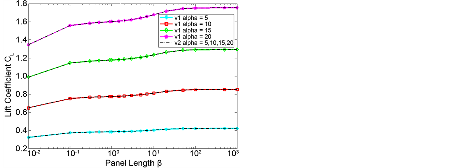
Figure 11. Results of CL vs β.

Figure 12. Converging time vs β for V∞ =10 [m/s] and α = 5 [˚].
the particular case of  [m/s] and α = 5 [˚]. The figure shows that as β decreases below the unit, the calculation times grows exponentially. In all the other studies conducted (for several
  and α), the results exhibited the same tendency.
4.3. Results for the γ Parameter
The γ parameter is related to the longitude of the wake and the wing, so it increases with each additional iteration. In Figure 13, the convergence of the obtained results of lift is displayed. In the figure are shown the results for the lower values of β, at the specific conditions of  [m/s] and α = 5 [˚].
The figure reveals that for β around the unit, the results converge quickly; however for panels with too small of a size, the program needs a lot more iterations to converge and the wake cannot be fully developed, which is why the computation times grows exponentially and the  is underestimated.
In Figure 14, the results for the second half of β values for the same study are observed. It shows how the wake can become thousands of times larger than the wing for panels that are too large. This affects the lift results because the wake behaves as a plane sheet causing the overestimated lift.
Given the results obtained of the study of panel size, the convergence, and computation time, the use of β between 0.3 and 2 and a wake length γ between 5

Figure 13. CL vs γ, V∞ =10 [m/s]; α = 5 [˚]; β between [0.01, 1.5].
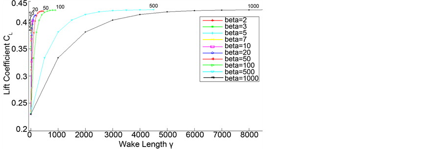
Figure 14. CL vs γ, V∞ =10 [m/s]; α = 5 [˚]; β between [2, 1000].
and 30 is recommended. Applying these conditions obtains accurate results, quicker convergence, and minimizes computation time.
These different results are only valid values for the geometric configuration studied, but certainly can serve as a reference for more complex study cases.
4.4. Results of CL vs α
In order to compare the results obtained by the panel method with those expected according to the lifting line theory, a graph that combines all results was made. Figure 15 presents a curve that summarizes all the results across  studies (red markers). The results for each angle of attack were averaged and the mean curve for
  vs α (green) was obtained. In addition, it is possible to see two segmented lines in the figure that correspond to the minimum and maximum value for each angle of attack; also, the theoretical 2D maximum lift curve (in blue) and the black line correspond to the expected results.
The results of lift coefficient for a plane wing obtained by the code implemented were compared with support values estimated by the lifting line theory and the results are similar.
The results follow the expected pattern of vorticity on the wing and the wake phenomena occurring in reality are observed, such as wingtip and start vortex. Given the convergence of the results, it is possible to state that the use of transient simulation wake is fully justified in aerodynamic systems using a setting that is appropriate for geometrical parameters. If the configuration is not suitable, it can incur in high times of unnecessary calculation.
5. Conclusions
The implementation of the free wake in the panel method faithfully represents the effects that occur in reality. In the wake, it is possible to distinguish wingtips vortex and start vortex generated by the profile out of the idle state.
By using suitable geometric parameters, the use of a transient wake configuration in the panel method is justified by the accuracy and the quick convergence of the results obtained.

Figure 15. Results of CL vs α.
By using a suitable position of the control panel on the wing, the occurrence of undesired phenomena in computing speeds induced on the wing trailing edge is avoided. These effects produce severe distortion of the panels and an excess of computed vorticity. The use of 0.25 times the wing chord is recommended.
The use of too long panels in the wake affects the circulation, the wake behaves as a plane sheet, and lift is overestimated. On the other hand, the use of too small panels requires many more iterations to converge the results and hence higher calculation times. To achieve good results and quick convergence, the use of β between 0.3 and 2, and γ between 5 and 30 is recommended.
The present work shows that the panel method is suitable for the prediction of lift on airfoils. The panel method implemented with transient wake turns out to be a good tool accessible to the academic level. In future studies using the panel method combined with other methods for predicting viscous effects, we will enhance the capabilities of the implemented method and produce a very good instrument for calculating the aerodynamic design of systems.
Acknowledgements
F.R.I. thanks everyone who helped to complete this work. Without their continued efforts and support, I would have not been able to bring my work to a successful completion. I wish to thank specially to Pablo Castillo and Castillo Capponi Aerospace for all the support and assistance provided.
Cite this paper
Fernando, R.I. and Pablo, C.C. (2017) Non-Dimensional Values for Convergence of Lift Prediction Us- ing Panel Method. Open Journal of Fluid Dynamics, 7, 26-39. https://doi.org/10.4236/ojfd.2017.71003
References
- 1. Stalewski, W. and Sznajder, J. (2010) Application of a Panel Method with Viscous-Inviscid Interaction for the Determination of Aerodynamic Characteristics of Cesar Baseline Aircraft. Institute of Aviation, Varsovia, 20.
http://ilot.edu.pl/prace_ilot/public/PDF/spis_zeszytow/207_2010/7_STALEWSKI_SZNAJDER.pdf - 2. Matos, D. (2012) Implementation of a 2D Panel Method for Potential Flow past Multi-Element Airfoil Configurations. Master in Mechanical Engineering. Thesis, Instituto Superior Técnico, Technical University of Lisbon.
- 3. Katz, J. and Plotkin, A. (1991) Low-Speed Aerodynamics: From Wing Theory to Panel Methods. Chaper, 12, McGraw-Hill, International Edition.
- 4. Woodward, F. (1968) Analysis and Design of Wing-Body Combinations at Subsonic and Supersonic Speeds. Journal of Aircraft, 5, 528-534.
http://arc.aiaa.org/doi/abs/10.2514/3.43979?journalCode=ja
https://doi.org/10.2514/3.43979 - 5. Carmichael, R. and Woodward, F. (1966) An Integrated Approach to the Analysis and Design of Wings and Wing-Body Combinations in Supersonic Flow. Ebook, California, 2-16.
http://ntrs.nasa.gov/archive/nasa/casi.ntrs.nasa.gov/19660029459.pdf - 6. Ramachandran, P., Rajan, S. and Ramakrishna, M. (2003) A Fast, Two-Dimensional Panel Method. SIAM Journal on Scientific Computing, 24, 1864-1878.
https://www.researchgate.net/publication/228742065_A_Fast_Two-Dimensional_Panel_Method
https://doi.org/10.1137/S1064827500374662 - 7. Falcão de Campos, J., Ferreira de Sousa, P. and Bosschers, J. (2006) A Verification Study on Low-Order Three-Dimensional Potential-Based Panel Codes. Computers & Fluids, 35, 61-73.
https://doi.org/10.1016/j.compfluid.2004.08.002 - 8. Willis, D. (2006) An Unsteady, Accelerated, High Order Panel Method with Vortex Particle Wakes. PhD Aeronautics and Astronautics. Massachusetts Institute of Technology Massachusetts.
- 9. Gaggero, S. and Brizzolara, S. (2008) A Potential Panel Method for the Prediction of Midchord Face and Back Cavitation. 6th International Conference on High Performance Marine Vehicles HIPER08, 1, 33-46.
http://www.hiper08.unina.it/cd%20hiper%2008/HTML/Papers/4%20-%20Gaggero%20Brizzolara.pdf - 10. Gaggero, S. and Brizzolara, S. (2008) A Potential Panel Method for the Analysis of Propellers in Unsteady Flow. 8th International Symposium on High Speed Marine Vehicles, HSMV08, 1, 115-123.
https://www.researchgate.net/publication/290543844_A_potential_panel_method_for_the_analysis_of_propellers_in_unsteady_flow - 11. Filkovic, D. (2008) Graduate Work. Master in Mechanical Engineering, University of Zagreb, Zagreb.
- 12. Prosser, D., Crassidis, A. and Ghosh, A. (2011) The Applicability of Unsteady Vortex Panel Methods to the Design of Hovering Flapping-Wing Micro Air Vehicles. AIAA Atmospheric Flight Mechanics Conference, Portland, 8-11 August 2011, 1-19.
http://enu.kz/repository/2011/AIAA-2011-6392.pdf - 13. Cox, C. (2011) Two Element Linear Strength Vortex Panel Method. Bachelor of Science in Aerospace Engineering. California Polytechnic State University, Obispo.
- 14. Van Garrel, A. (2011) Development of a Wind Turbine Rotor Flow Panel Method. Energy Research Centre of the Netherlands, 1-52.
http://www.ecn.nl/docs/library/report/2011/e11071.pdf - 15. Santana, L., Schram, C. and Desmet, W. (2012) Panel Method for Turbulence-Airfoil Interaction Noise Prediction. 33rd AIAA Aeroacoustics Conference, Colorado Springs, 4-6 June 2012, 1-10.
https://lirias.kuleuven.be/bitstream/123456789/360491/1/AIAA-2012-2073-528.pdf - 16. Tarafder, M., Ali, M. and Nizam, M. (2013) Numerical Prediction of Wave-Making Resistance of Pentamaran in Unbounded Water Using a Surface Panel Method. Procedia Engineering, 56, 287-296.
https://doi.org/10.1016/j.proeng.2013.03.120 - 17. Tan, J. and Wang, H. (2013) Panel/Full-Span Free-Wake Coupled Method for Unsteady Aerodynamics of Helicopter Rotor Blade. Chinese Journal of Aeronautics, 26, 535-543.
https://doi.org/10.1016/j.cja.2013.04.050 - 18. Fernandes, J. (2013) Construção de uma Ferramenta Computacional para a Simulação Aerodinamica de um conjunto Asa e Flap. Master en Ingenieríaaeroespacial. Instituto Superior Tecnico, Lisboa.
- 19. Erickson, L. (1990) Panel Methods—An Introduction. NASA Ames Research Center, Moffett Field. http://ntrs.nasa.gov/search.jsp?R=19910009745
- 20. Atassi, H. (2016) The Biot-Savart Law. Professor Atassi Teaching, University of Notre Dame, Notre Dame.
https://www3.nd.edu/~atassi/Teaching/ame%2060639/Notes/biotsavart.pdf