Open Journal of Fluid Dynamics
Vol.04 No.01(2014), Article ID:43397,25 pages
10.4236/ojfd.2014.41003
Investigation of Wave-Structure Interaction using State of the Art CFD Techniques
Jan Westphalen1, Deborah M. Greaves1, Alison Raby1, Zheng Zheng Hu1, Derek M. Causon2, Clive G. Mingham2, Pourya Omidvar3, Peter K. Stansby3, Benedict D. Rogers3
1School of Marine Science and Engineering, Marine Institute, University of Plymouth, Plymouth, UK
2School of Computing, Mathematics and Digital Technology, Manchester Metropolitan University, Manchester, UK
3School of Mechanical, Aerospace and Civil Engineering, University of Manchester, Manchester, UK
Email: deborah.greaves@plymouth.ac.uk
Copyright © 2014 by authors and Scientific Research Publishing Inc.
This work is licensed under the Creative Commons Attribution International License (CC BY).
http://creativecommons.org/licenses/by/4.0/


Received 21 December 2013; revised 21 January 2014; accepted 29 January 2014
ABSTRACT
The suitability of computational fluid dynamics (CFD) for marine renewable energy research and development and in particular for simulating extreme wave interaction with a wave energy converter (WEC) is considered. Fully nonlinear time domain CFD is often considered to be an expensive and computationally intensive option for marine hydrodynamics and frequency-based methods are traditionally preferred by the industry. However, CFD models capture more of the physics of wave-structure interaction, and whereas traditional frequency domain approaches are restricted to linear motions, fully nonlinear CFD can simulate wave breaking and overtopping. Furthermore, with continuing advances in computing power and speed and the development of new algorithms for CFD, it is becoming a more popular option for design applications in the marine environment. In this work, different CFD approaches of increasing novelty are assessed: two commercial CFD packages incorporating recent advances in high resolution free surface flow simulation; a finite volume based Euler equation model with a shock capturing technique for the free surface; and meshless Smoothed Particle Hydrodynamics (SPH) method. These different approaches to fully nonlinear time domain simulation of free surface flow and wave structure interaction are applied to test cases of increasing complexity and the results compared with experimental data. Results are presented for regular wave interaction with a fixed horizontal cylinder, wave generation by a cone in driven vertical motion at the free surface and extreme wave interaction with a bobbing float (The Manchester Bobber WEC). The numerical results generally show good agreement with the physical experiments and simulate the wave-structure interaction and wave loading satisfactorily. The grid-based methods are shown to be generally less able than the meshless SPH to capture jet formation at the face of the cone, the resolution of the jet being grid dependent.
Keywords:
Wave Loading; Wave Energy; Wave-Structure Interaction; Manchester Bobber; CFD; Physical Experiments; FV; CV-FE; SPH; Cartesian-Cut-Cell; SPHysics; AMAZON SC; STAR CCM+; CFX

1. Introduction
In the design of floating offshore WEC structures, many of the same engineering issues arise as for floating offshore structures used in the oil and gas industry. There are some similarities between the design challenges in the two industries and some of the techniques and tools developed within the oil and gas sector can be applied to wave energy. However, there are also significant differences. WECs are usually designed to have moving parts that react to wave motion; WECs are generally much smaller than offshore structures; the water depth is usually shallower and WECs are generally expected to be deployed in arrays, so the design is not a “one off”. The structural design of offshore floating wave energy converters (WECs) generally involves three main and interacting parts of the device: the floating absorber, the mooring arrangement and the power-take-off (PTO) with its associated control system.
Unlike large offshore structures in which motions and forces are minimised, WECs are designed to perform large motions in small and intermediate seas for efficient power conversion, but to survive extreme waves in the event of a storm. These design parameters require mooring arrangements that hold the device in place but do not restrict the motion of the WEC in its energy capturing mode. The dynamics of the moorings, including the motion of the cables, risers, weights and floats, may be highly non-linear in terms of hydrodynamic and structural interaction, and this can affect the response of the device negatively (or positively). The PTO system, however, directly affects the dynamics of the WEC as it converts energy.
In the engineering design of WECs, the three areas of device hydrodynamics, mooring and PTO/control strategy can affect each other considerably and therefore should be considered together. The hydrodynamics can be described using the equations of motion to represent, for example, a single-body heaving device as a mass-spring-damper system, in which the mooring forces are included in the system stiffness and the PTO forces as external forces. Added mass and damping are shape and frequency dependent and can be evaluated using standard naval architecture techniques by physical tank tests, or by numerical methods, which solve the initial boundary value problem for radiation and diffraction for a given geometry [1] [2] . The assumptions for these numerical methods to be valid are: irrotational, inviscid fluid flow, linear wave theory and small body motion. By construct, in the frequency domain the waves are monochromatic and sinusoidal, which limits their applicability for a WEC in real sea conditions.
Modelling in the time domain is necessary for WEC control studies and for investigation of nonlinear wave interaction. Cummins [3] converted the frequency domain coefficients in the time domain by calculating impulse response functions (IRF). The IRF describes the response of the system after an initial impulse and can be used in the time-domain formulation of the equations of motion. With this approach it is possible to simulate polychromatic seas. However, the same assumptions of linear theory and irrotational, inviscid fluid flow apply. When several waves are superposed, these assumptions can be violated, as waves may become large, and especially when the wave frequency is close to the natural frequency of the WEC, unrealistically large body motions may occur because friction and viscous losses are not usually taken into account.
Here, we focus on the hydrodynamics of the WEC body and its interaction with an extreme wave and investigate a hierarchy of CFD approaches applied to this case. The design of the WEC with regards to its survivability demands a nonlinear description of the hydrodynamics. Here, steep and large waves that can generate significant water impact on the structure need to be modelled. This may involve wave breaking and green water on the deck of the device. Viscous effects may become large and also the body motions may become highly non-linear, as a floating device can become fully submerged or airborne.
As argued above, when investigating the hydrodynamics of extreme wave-structure interaction, linear theory is of uncertain accuracy and fully non-linear numerical methods are required. Mathematically, such problems can be described by the Navier-Stokes equations incorporating a free surface. These include viscous effects and, depending on the discretisation of the equations, surface effects such as wave breaking can be simulated. When viscous effects are judged to be not important and are neglected, the Navier-Stokes equations reduce to the Euler equations. Both sets of equations can be discretised on a two- or three-dimensional mesh and numerical techniques such as the well-known Finite Volume (FV) or Finite Element (FE) formulations can be used to compute the fluid velocities and pressures at every mesh cell or node. Bodies can be modelled as cavities in the mesh and body motion can be simulated by dynamic body fitted meshes. Special attention needs to be taken when modelling the free surface motions, and Lagrangian surface tracking or Eulerian surface capturing may be used. The volume of fluid (VoF) surface capturing method is often used in CFD and involves the introduction of an additional variable, the volume fraction, which is advected with the flow and represents the fraction of water in a given cell. At the free surface, cells are partially filled and the volume fraction lies between 0 and 1. This approach has been used successfully to simulate the motions of a ship in waves, as reported by Hadzic et al. [4] . The alternatives to the Eulerian grid-based methods are Lagrangian methods such as Smoothed Particle hydrodynamics (SPH); these are meshless methods and do not require special treatment of a free surface.
In this paper we use three Eulerian based methods, two that solve the Navier-Stokes equations and one the Euler equations on a three dimensional mesh, and Lagrangian SPH methods. All of the techniques are used to simulate fluid structure interaction problems of increasing complexity. First, a fixed horizontal cylinder in regular waves is modelled. The time histories of the vertical forces are compared to physical experiments and potential theory [5] . The next experiment is a cone in vertical motion that radiates waves at the still water surface. It follows a prescribed displacement of the form of a Gaussian wave packet [6] .
The last set of results compares the motions of a freely floating body interacting with extreme large waves and a counterweight, which is connected to the main float by a pulley-rope system. This case shows the capabilities of the three Eulerian CFD methods to simulate a floating body in one and two degrees of freedom in very non-linear waves, but also the interaction with a counterweight. This counterweight is represented by a force acting on the body, which can provide an option to also include non-linear PTO and mooring forces, for example to test controllers or evaluate non-linear hydrodynamic interaction between the main device and its auxiliaries.
Section 2 describes the three CFD approaches used here, namely the Navier-Stokes/Finite Volume, the Euler/ Cartesian-Cut-Cell and SPH solvers. The test cases including the results are described in Section 3 and conclusions are discussed in Section 4.
2. Numerical Models
2.1. Finite Volume (FV) Method
The Finite Volume solver [7] is indicated by the acronym CV and refers to the commercial code STAR-CCM+. It uses the Navier-Stokes equations discretised on a 3-dimensional mesh to calculate the velocities and pressures in the flow field in a segregated iterative way. The domain, here a numerical wave tank (NWT) including the structure, such as a horizontal cylinder, is subdivided into discrete volumes. The surface and volume integrals performed on the control volumes are used to calculate the solution variable values at the centre node of each CV as illustrated in Figure 1 [8] The variables are stored in a collocated manner, such that the pressures and velocities are computed at the same locations. To avoid the so-called “checker-board” effect, which might occur for non-staggered variable arrangements [9] , the pressures and velocities are calculated using a segregated iterative approach [10] .
Free surface calculations are performed using the VoF method [11] and an additional equation for advection of the volume fraction, c, is solved. For a CV that is fully filled with water, the volume fraction, c = 1.0; when empty of water, the volume fraction c = 0; for cells at the interface containing fractions of both fluids, the sum of both fractions is unity. To find the location of the water surface, which is taken as the iso-value of the water fraction c = 0.5, a high resolution interface capturing scheme (HRIC) is applied. This is dependent on the local Courant number of the cell and thereby on the time step. It is similar to the compressive interface capturing scheme for arbitrary meshes (CICSAM) [8] [12] - [14] .
Meshes comprising hexahedral cells are used for the simulations presented here. A typical mesh section can be seen in Figure 2(a). The cells are refined in steps of two, so that one coarse cell is split into two smaller cells occupying the same face length in two dimensions. Figure 2(b) shows the mesh close to the boundary of a cylinder, which is modelled as a cavity in the mesh. Prism layers are used to resolve the hydrodynamics in the vicinity of the surface properly. Where the boundary-fitted prism layers meet the rest of the mesh, arbitrary cell

Figure 1. Arrangement of velocity components on a control volume element of a structured grid at the central node, element faces, and element vertices.

 (a) (b)
Figure 2. Mesh refinement (a) and prism layer close to a body, modelled as a cavity (b).
shapes occur, as the boundary-fitted mesh structure is effectively cut out of the initially hexahedral mesh.
When mesh motion is included in the simulation, as for the single float in extreme waves described in Section 4, the whole domain is displaced according to the motion of the float. Thus, the connectivity of this mesh is fixed, the cut cells are not recomputed and re-meshing or dynamic meshing is not necessary at each time step. The mesh motion is taken into account by calculating the face velocities required in the discretisation of the governing equations as the difference between the fluid velocity and the face velocity resulting from the mesh motion.
2.2. Control-Volume Finite Element (CV-FE) Method
The Control-Volume Finite Element (CV-FE) approach [15] used here is the commercial package ANSYS CFX. It combines the Finite Volume method’s control volume formulation with the Finite Element method by using shape functions and a vertex-centred discretisation scheme. The shape functions are used to describe the distribution of a variable across the CV [15] - [17] . As described for the Finite Volume method in the previous section, the CV-FE also solves the Navier-Stokes equations. The general transport is discretised using a collocated variable arrangement on a 3-dimensional grid containing hexahedral cells. The CVs are arranged around the mesh nodes (vertex-centred) as shown in Figure 3 and thereby this technique ensures the conservation of flow quantities such as mass and momentum.
As above, the volume fraction field is solved using the VoF formulation [10] . However, in the CV-FE approach, the fluid interface is calculated using a compressive interface capturing scheme [15] [18] - [20] , which is dependent on the filling level of the surrounding cells rather than the Courant number as is the case for CICSAM
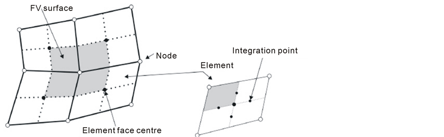
Figure 3. Vertex-centred discretisation of variables for Navier-Stokes/CV-FE solver.
[12] . This means that the resolution of the fluid interface is time step independent and allows for larger time steps. The discretised equations are solved using a fully coupled system of linear equations, in which the pressure and velocity are linked to avoid decoupling and non-physical solutions that may otherwise occur [21] .
In Figure 4(a), a typical mesh used for the CV-FE solver is shown, in which meshes with only hexahedral cells are used. In two dimensions, the cell refinement divides each cell into three, and creates transition layers such that each cell face coincides with one cell face on the refined side. A structure in the domain is represented using a body-fitted mesh of hexahedral cells, which may be distorted close to the structure boundary as seen in Figure 4(b). This may influence the initial solution of the free surface, if it cuts through these distorted cells. For cases involving body motion, the mesh is moved at each time step by moving the nodes and edges of the mesh according to the local velocity field, before the fluid dynamics equations are solved. In this way, the mesh connectivity is not changed, but the mesh cells are stretched.
2.3. Smoothed Particle Hydrodynamics
Smoothed Particle Hydrodynamics (SPH) is a flexible Lagrangian and meshless technique for CFD simulations that can be used in complex problems. In this method the fluid system is represented by a set of particles which have individual material properties and move according to governing conservation equations [22] . In the Lagrangian method, any flow variable is expressed as , where x is the point vector of the particle at the reference time t =0.
The major advantage of using SPH is in dealing with large deformations and distorted free-surface problems. There is no mesh construction in SPH, therefore in certain problems, for instance simulation of waves, the SPH method may be easier to develop and use than Eulerian methods. Also, there is no need for special treatment of the free surface in order to simulate highly nonlinear and potentially violent flows, such as breaking waves. Furthermore, the equations used in SPH are quite simple in comparison with other methods. However, the computational cost is one of the disadvantages of SPH; the time step is much smaller than other methods due to using an explicit time integration scheme.
Following the work of [23] , the governing equations for compressible flow are solved in conservative form with an Arbitrary-Lagrangian Eulerian (ALE) SPH scheme. Here, a Riemann solver is used for each particle-particle interaction since pressure fields can be predicted satisfactorily and the classical SPH formulation may cause propagating waves to decay in the channel [24] . The interaction between each particle pair is solved as a 1-D Riemann problem. Herein, we use a parallel version of the SPHysics code [24] where this Riemann problem is solved using an HLLC approximate Riemann solver with MUSCL-based upwinding [25] and a β-limiter [26] [27] .
The SPHysics code [28] has a choice of kernel function. Here, we use the cubic kernel function, which is found to be the best choice for propagation of waves in a channel [22] . The cubic kernel is known to exhibit tensile instability, and has to be corrected, according to [27] in order to avoid particle clumping. The symplectic algorithm [22] [28] , often known as kick-drift-kick, is used as the time stepping method. Here, kick is the change in velocity v by the force and drift is the change in coordinate, r.
The repulsive force boundary condition [28] [29] , uses boundary particles to exert forces on fluid particles according to a specified function acting normal to the wall. Boundary particles experience an equal and opposite

 (a) (b)
Figure 4. Mesh refinement (a) and body-fitted mesh close to the structure, modelled as a cavity (b).
force to the repulsive force that they exert on surrounding fluid particles. Based on the technique of Monaghan et al. [29] for simulation of rigid floating bodies, the force on each boundary particle is computed by summing up the contribution from all the surrounding water particles within its kernel. The boundary particles within the rigid body are then moved by integrating in time the equations of motion of the body in the translational and rotational degrees of freedom. It can be shown that this technique conserves both linear and angular momentum [22] [29] .
2.4. Incompressible SPH (ISPH)
For virtually incompressible flows such as water the divergence free condition for continuity may be directly imposed by the projection method of Chorin [30] , first applied by Cummins and Rudman [31] in SPH. This has the advantage of much reduced pressure noise, larger time steps, improved accuracy but the disadvantage of a Poisson solver for pressure. The present method is described by Lind et al. [32] with some improvements by Skillen et al. [33] . A second-order time marching scheme is applied, where both the density and mass of the incompressible particles are constant and the stabilised bi-conjugate gradient method is used to solve the linear system that results from the discretised form of the pressure Poisson equation.
There is a further difficulty associated with highly accurate ISPH; instability can occur due to particle clustering, e.g. near stagnation points. This may be avoided without loss of accuracy or convergence by particle shifting, equivalent to remeshing. This may be slight shifting across streamlines [34] or more generally by Fickian shifting along lines of decreasing particle density [32] which is suited to free surface flows.
2.5. Cartesian Cut Cell Method
The AMAZON-3D numerical wave tank (NWT) is based on the free surface capturing method for two fluid flows with moving bodies developed by Qian et al. [35] , in which is demonstrated a rigid 2D wedge-shaped body entering and exiting calm water including total immersion. The AMAZON-3D code uses a Cartesian cut cell method to provide a boundary-fitted grid for both static and moving boundaries in 3D. The main advantages of the Cartesian cut cell approach have been outlined previously [36] [37] , including particularly its flexibility for dealing with complex geometries and moving bodies. There is no requirement to re-mesh globally or even locally for a moving boundary problem which only requires changes locally at cells in the background Cartesian mesh that are cut by the moving boundary contour.
The AMAZON-3D code is based on the integral form of the Euler equations for 3D incompressible flow with variable density. The free surface is treated as a contact surface in the density field that is captured automatically during a time-marched calculation without special provision in a manner analogous to shock capturing in compressible flow. A time-accurate artificial compressibility method and high resolution Godunov-type scheme replaces the pressure correction solver used in many current VoF methods. AMAZON-SC can handle break-up and recombination of the free surface as well as air entrainment into the water and, in principle, associated local compressibility effects. The total force is obtained by integration of the pressure field along the body given by
 , where
  is the body surface and is defined by the cut cell surface.
3. Results
In order to assess the suitability of the four different CFD approaches to simulate WEC survivability design scenarios, they are applied to a series of benchmark test cases of increasing complexity. In each case, data from physical experiments are available and used for comparison. Grid convergence has been studied in comparisons of free surface wave simulations using FV and CV-FE, in which regular waves are simulated by using different meshes of hexahedral, polyhedral and tetrahedral shape with different resolution and is summarized in [38] ].
3.1. Fixed Horizontal Cylinder in Regular Waves
Dixon et al. [5] carried out physical tank tests in order to improve Morison’s formula for the calculation of the forces on a horizontal cylinder. For different levels of cylinder submergence and different wave amplitudes the vertical forces acting on the cylinder in waves were recorded. Here, the four CFD techniques are applied to a selection of these tests and compared with the experimental results.
The forces calculated using each of FV, CV-FE, SPH and AMAZON are compared for different wave amplitudes and cylinder axis depths. The properties including the position of the cylinder below still water level, d, the wave steepness, kA, the product of the wave number and water depth, kh and the Keulegan-Carpenter number KC for each case are summarised in Table 1. The relative amplitude A' and axis depth, d', are non-dimen- sionalised by the cylinder diameter D. To compare the numerical results with those obtained by Dixon et al. [5] , the vertical forces, Fz, on the cylinder resulting from drag and pressure on the surface are derived. In the physical experiments, the forces were measured over one wave cycle. The force predicted by the CFD methods once steady-state was reached, Fz, is non-dimensionalised using the following expression
 (30)
(30)
with Fz being the measured vertical force on the cylinder, g, the acceleration due to gravity, ρ, the density of water, D, the cylinder diameter and l, the length of the cylinder.
As in the physical experiments, linear regular waves are generated in the NWT to interact with the structure. For the Eulerian grid-based approaches described in Sections 2.1, 2.2 and 2.4, the wave velocity components u and w and the surface elevation η are described by
 (31)
(31)
 (32)
(32)
and
 (33)
(33)
and are applied to the water component at the upstream end of the 3-dimensional NWT using a velocity inlet boundary condition. The velocities for the air component are set to 0.0 m/s. The top boundary is a pressure outlet, the sides are modelled as symmetry planes and the bottom, the cylinder boundary and the downstream end of the domain are defined as walls. The total number of cells for the FV meshes is approximately 114,599 and the CV-FE meshes contain approximately 695,375 cells. The number of cells on the boundary of the cylinder itself, however, is 250 for the FV solver and 236 for CV-FE. The time step to achieve a converged solution is found to be 0.001 s and 0.005 s for FV and CV-FE respectively. Details of the NWT for each of the codes used are summarised in Table 2.

Table 1. Properties of horizontal cylinder cases.
Table 2. Details of the NWT used by each code for the horizontal cylinder cases.
In AMAZON SC, the air part of the left-hand boundary and the top and right boundary are specified as non-reflecting boundary conditions allowing air to leave or enter the domain. ditions allowing air to leave or enter the domain. The cylinder surface is defined as a reflective wall boundary. The remaining sides are slip boundaries. The NWT contains approximately 458,850 cells with a minimum edge length of 0.015 m. A time step of 0.00025s is applied. For the SPH method the calculations are carried out in a 2-dimensional NWT using 7800 particles in the domain. The boundaries at the wave maker, the bottom, the downstream end and the cylinder are treated as walls and waves are generated by moving the upstream wall similar to a piston wave maker.
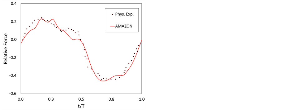
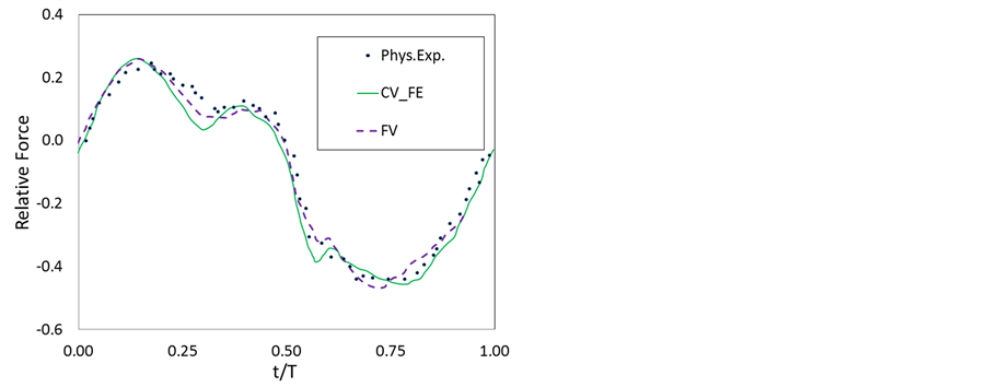
In Figures 5 and 6 the time-histories of the non-dimensionalised vertical forces, F', over one wave period are shown for all solvers. For the mesh methods, both mesh and time step convergence are achieved for the results presented. The ISPH method is converged regarding the number of particles in the NWT and the time step. Con- vergence studies for the different CFD approaches are reported in the literature [35] [39] [40] . It was found by Westphalen et al. [39] that 14 cells in the vertical direction are sufficient to resolve the free surface accurately.
For case 1, d' = 0.0 and A' = 0.5, the three codes give very good agreement with the experimental data. The CV-FE results follow the experimental data well and the FV also agrees well, although a third peak is evident in the numerical result but not visible in the experiment data. The AMAZON SC result also represents the force characteristic reasonably well, although the second peak is not resolved well and occurs late and reduced in size, however, the second trough is generally well reproduced. The ISPH result gives a slightly noisy signal and the first trough is shallower and offset compared with the experiment, but the general trend is in reasonable agreement with the other data. For case 2, d' = −0.3 and A'= 0.2 the results look even better and each of the mesh-based solutions follows the experimental data well and reproduces the observed characteristics. As before, the ISPH results are noisier than the other techniques and this is would be reduced by increasing particle resolution but with increasing computational cost. Table 2 gives details of the CPU run time and computer architecture used by each of the codes.
Figure 7 shows snapshots of the surface elevation around the cylinder for case 1 (d' = 0.0) at different times calculated by the FV solver and the AMAZON code. The different codes show similar free surface behaviour at each time step, with overtopping of the cylinder t/T = 0.36. At time step, t/T = 0.6, air entrainment can be observed in the FV solution. Figure 8 shows the free surface profile in the tank and particle distributions calculated using the ISPH method at two different time instants for case 1. The solution in Figure 8(a) is at a time instant between those in Figures 7(i) and (j), and Figure 8(b) corresponds with Figure 7(l). The wave propagation near the cylinder has clearly been altered by the presence of the cylinder. Since the ISPH simulations are mono-phase (i.e. only water particles) the compressibility of air around the cylinder is not taken into account.
 (a) (b)
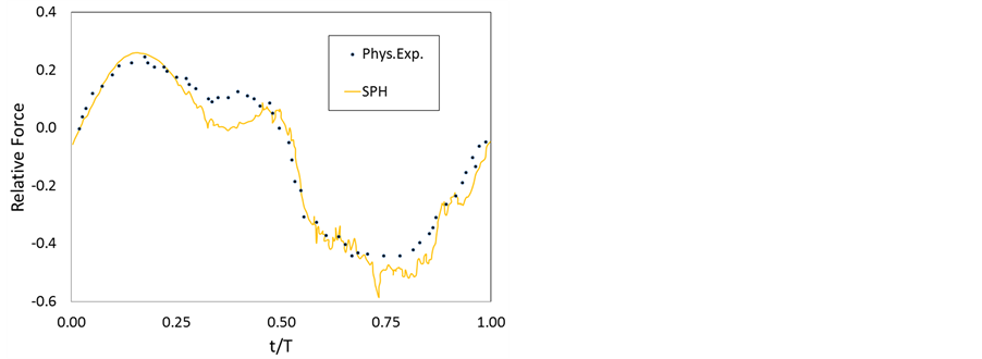 (c)
(c)
Figure 5. Relative vertical forces on horizontal cylinder, Case 1 (d' = 0.0, A' = 0.5); a) CV_FE and FV, b) AMAZON, c) SPH.
The cylinder is half submerged in case 1 and three quarters submerged in case 2 and the wave amplitude in case 1 is larger than in case 2, such that the wave overtops the cylinder in case 1 but not in case 2. Thus, it is to be expected that the results predicted by the numerical codes for the less challenging case 2 will be better than those for case 1 in which wetting and drying of the cylinder occurs, as seen in Figures 7 and 8.
3.2. Driven Motion: Oscillating Cone in Still Water
For the simulation of floating bodies, the eventual aim is to simulate the motion of floating WECs in extreme waves, and thus it is important to be able to calculate the forces on a moving body and the surface elevations around it correctly. For the second test case, a cone shaped body positioned with its vertex at the initially still water surface is chosen, for which physical tank tests are described by Drake et al. [6] . The motion of the cone is driven and not influenced by the forces generated on its surface by the surrounding fluids. In the experiments, the vertical forces on the cone surface due to its motion and the relative water surface elevation at a distance of 0.02 m from the cone surface are recorded. Here, comparisons between AMAZON, the CV-FE solver, SPH and the physical experiments are shown.
The motion of the cone is defined by the displacement d(t) from the initial position at t = 0 s following the form of a Gaussian wave packet, which is described by
 (34)
(34)

 (a) (b)
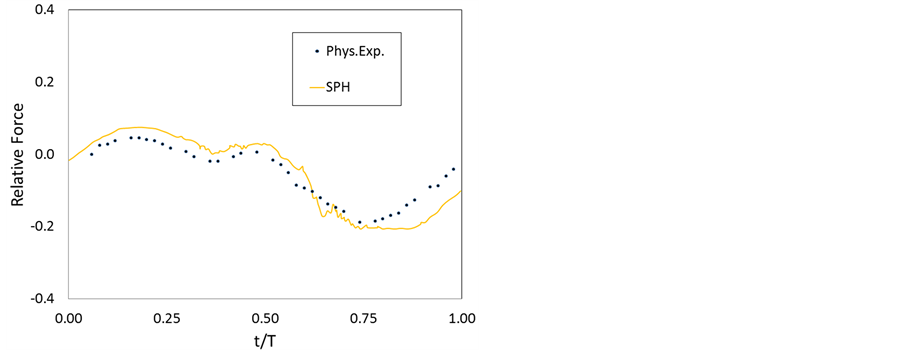 (c)
(c)
Figure 6. Relative vertical forces on horizontal cylinder, Case 2 (d' = −0.3, A'=0.2);a) CV_FE and FV, b) AMAZON, c) SPH.
where
 (35)
(35)
with h = 0 or 1. A denotes the largest excursion from the still water level. N is the number of frequency components and ωn is the appropriate circular frequency. The central circular frequency ω0 [rad/s] is defined by
 (36)
(36)
with m being an integer between 1 and 12. m effectively controls the linearity of the case. The larger m is and thereby the central frequency, the more non-linear the dynamics become. The results presented here are for h = 1, m = 6 and 9 and A = 0.05 m.
For the CV-FE approach the simulations are performed in a three-dimensional domain with a length and width of 2.5 m and a height of 2.0 m. The cone is placed in the centre, as can be seen in Figure 9 and has a maximum diameter equal to 0.6 m and a dead rise angle of 45˚. The slope itself is 0.3m high. The initial draught of the cone is 0.15 m at a water depth of 1.0 m. The cone is modelled as a cavity in the mesh. The outer boundaries, the bottom of the tank and the cone are modelled as free slip walls. The top boundary is defined as a

 (a) (b) (c) (d) (e) (f)

 (g) (h) (i)
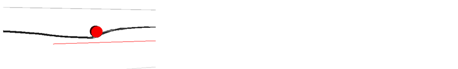

 (h) (k) (l)
Figure 7. Snapshots of surface elevation (a-f: FV and second group: g-l: AMAZON), case. d' = 0.0, A' = 0.5; (a,g) t/T = 0.0, (b,h) t/T = 0.12, (c,i) t/T = 0.36, (d,j) t/T = 0.6, (e,k) t/T = 0.73, (f,l) t/T = 1.0.
 (a)
(a) (b)
(b)
Figure 8. Particle configuration for half submerged cylinder (SPH). (a) t/T = 3.5; (b) t/T = 5.0.
pressure outlet with constant atmospheric pressure. The mesh consists of 820,000 hexahedral cells, where the regions around the water surface and the cone surface are highly refined to achieve cell edges of approximately 0.01 m. The outer regions are relatively coarse to save computational resources and encourage numerical damping, thus avoiding reflections from the walls. The simulations were carried out using a high performance computing, HPC, cluster on 16 CPUs. The time step is 0.0005 s. Details of the CPU run time and computer architecture used by each of the codes for this case are summarised in Table 3.
For the AMAZON simulations a 2 m × 1.6 m axisymmetric domain is used. The still water level is set to 1.0 m and the initial draught of the cone is 0.148 m. The calculations are performed on a hexahedral grid using an axisymmetric (2D) version of the code with cell sizes of 0.01 × 0.01 m. The time step is 0.00005 s.
The exported vertical forces Fz from the CFD codes are non-dimensionalised using the expression
 (37)
(37)
with ρ being the density of fresh water, g the acceleration due to gravity, r the cone radius at still water level and A the maximum excursion. Also the time is divided by the corresponding period of the central frequency ω0. The
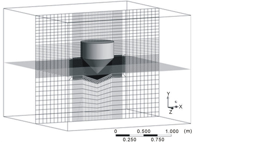
Figure 9. Domain for the oscillating cone case with a section of the mesh at the centreline. The dark region close to the body shows the highly refined mesh, which was necessary to capture the surface jet effects.
Table 3. Details of the NWT used by each code for the oscillating cone case.
measured relative motion of the water surface is divided though the maximum excursion A = 0.05 m.
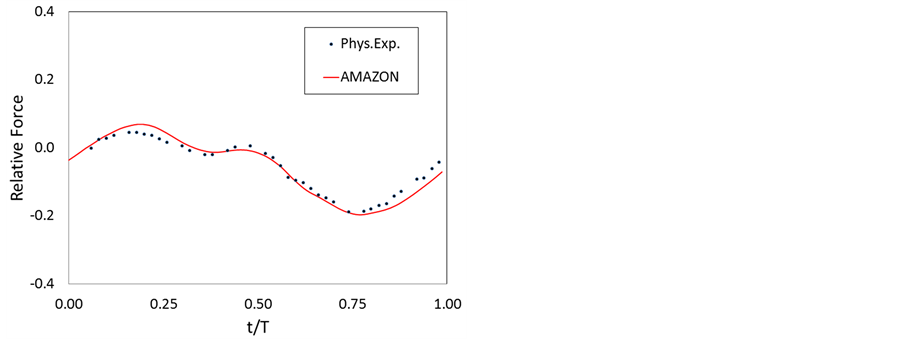
Figure 10 compares the force data obtained by the three CFD methods with those of the physical experiments in which m = 9. Here, t/T = 0 corresponds to the instant when the vertical impact force is maximum. It is so chosen because different simulations have a different starting time, e.g., for the AMAZON code simulations, t is time from zero and to = total time/2 in Equation (34), where the total time is defined to be 8T = 5.333 s for the case in which m = 9, and therefore, (t-to) is negative. Generally the agreement between numerical prediction and physical experiment is satisfactory. The Eulerian techniques generate little differences especially in the force minima and maxima. AMAZON slightly overestimates the forces and the Navier-Stokes solver underestimates them. The Lagrangian SPH method also agrees well although the troughs are less well resolved.
For the solution of the relative motion of the free surface at the cone, shown in Figure 11, greater differences between the numerical predictions and experiments are evident. Here, the mesh-based AMAZON and CV-FE methods produce results that under-predict the peak values and predict shallower troughs than were measured in the experiment. The particle-based SPH results, however, generally agree very well with measured free surface position at the cone edge, although the predicted troughs are deeper. The difficulty with capturing the free surface close to the cone is due to the occurrence of a jet-effect. This is not apparent for cone cases with low central frequency, where the relative motion of the surface elevation is resolved better.
The grid convergence index (GCI) has been examined for the AMAZON code and results shown in Figure 12. For three levels of mesh resolution (mesh 1 represents the finest mesh with dx = dy = 0.01 m, mesh 2 represents dx = dy = 0.02 m and mesh 3 represents dx = dy = 0.04 m), the RMS of the non-dimensionalized vertical forces
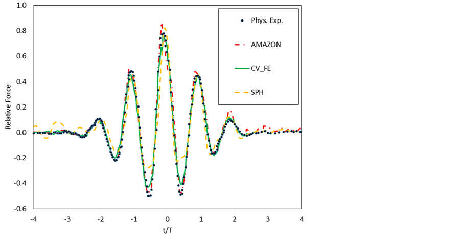
Figure 10. Relative vertical force on cone, m = 9.

Figure 11. Relative surface motion at cone, m = 9.
are 0.3387, 0.3400 and 0.3475 respectively, from which it can be calculated that the value of GCI32 is approximately 0.9% and GCI21 is 0.16%. For the SPH code, results for the grid convergence study are shown in Figure 13. Two levels of resolution are tested; particle spacing, Δ = 0.02 m and Δ = 0.04 m. The RMS of the non-dimensionalized vertical forces are 0.281 and 0.258 respectively, from which it can be calculated that the value of GCI21 is approximately 0.5%.
Using the CV-FE approach, simulations have been carried out in pairs in order to consider the positive direction cone displacement for a maximum excursion of A = +50 mm and the opposite negative displacement for A = ‒50 mm. To analyse the nonlinearity in the case, the time histories of the relative surface elevations for the paired tests, m = 9, have been subtracted and summed respectively and divided by 2. This enables results to be broken down into linear and higher order components and compared separately. The half-sum is given by
 (38)
(38)
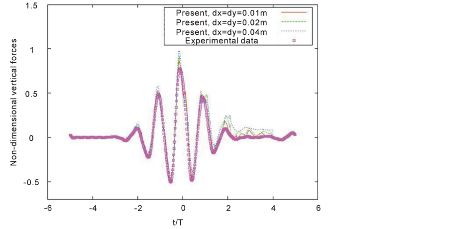
Figure 12. Grid convergence of AMAZON code for relative vertical force on cone.
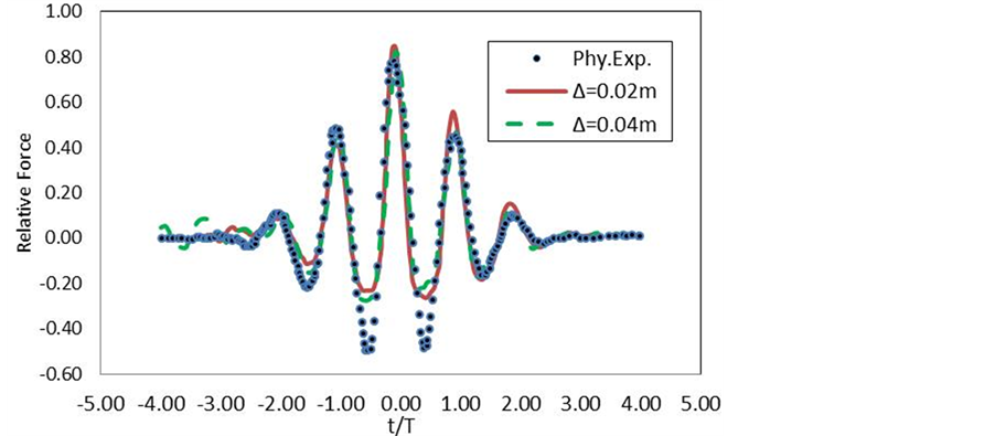
Figure 13. Grid convergence of SPH code for relative vertical force on cone.
and the half-difference by
 , (39)
where C and T are the solutions for crest focussed and trough focussed cases. When the half-sum is calculated, the odd frequency components cancel out and the even frequency components remain, and the results of this manipulation on the predicted surface elevations for m = 9 are plotted in Figure 14. Thus the sum line in Figure 14 is composed of second and higher order even frequency components and is dominated by the second order terms; similarly when the half-difference is calculated, the even terms are removed and the odd frequency components remain and are dominated by the linear component, shown in the difference line in Figure 14. For the central circular frequency corresponding to m = 9 the relative water surface elevation clearly contains a higher order component represented by the solid line. Unlike the linear part the higher order component is not symmetric about the mean water line. It oscillates with double the frequency of the linear part around a slightly raised water level.

Figure 14. Surface elevation: half-sum and half-difference comparison (m = 9).
Applying the same analysis technique for the vertical forces, results in the plots shown in Figure 15. Here, the higher order parts, i.e. the sum terms, have a double frequency component superimposed on an asymmetric positive component. The total force may be further decomposed into its hydrostatic and hydrodynamic parts. The hydrostatic part results from the buoyancy force, which is subtracted from the total force to obtain the hydrodynamic contribution. Figure 16 shows the non-dimensionalised vertical forces for m = 9 for the maximum excursion negative case, decomposed into dynamic and hydrostatic components. For the lower frequency case, m = 6, the same plot is shown in Figure 17. Here, the hydrodynamic force is a much smaller component of the total force. This is because, due to the higher central circular frequency for larger m, the Keulegan-Carpenter number, KC, reduces; KC is given by
 , (40)
where A is the maximum excursion, Tω0 the period corresponding to the central frequency and d is the diameter of the cone at the still water level. KC describes the relationship between the drag forces over the inertia. For lower KC the inertia dominates the force contribution. This can be seen in the results. For case m = 9, with KC = 0.11, the dynamic force component, which is related to the inertia of the cone, is more developed than for case m = 6, with KC = 0.16.
3.3. Floating Body Motion: Manchester Bobber in extreme waves
Physical tank testing of the Manchester Bobber device at 70th scale was performed in the wave tank at the University of Manchester. It is 18.5 m long, 5 m wide and tests were carried out in a water depth of 0.5 m. The waves are generated using 8 piston type paddles operated using the Edinburgh Designs “OCEAN” interface. To minimise reflections from the far end wall, a curved surface piercing beach is installed [41] [42] .
Here, tests for a single tethered float are reproduced using two Eulerian approaches; the Euler/Cartesian- Cut-Cell and Navier-Stokes/FV Method. A schematic arrangement of the system can be seen in Figure 18, where mf and mc are the masses of the float and the counterweight respectively. The horizontal displacement of the float is restricted due to the vertical cables. These are attached to the superstructure and held taut by weights at their ends. In the physical experiments vertical displacements are deduced from the angular displacement of the pulley ωp. During all tests no power was taken off the system and the friction in the pulley support is negligible. The cables are assumed to be stiff and inextensible. Further details on the experimental system are given by Stallard et al. [41] and Weller et al. [42] for a different float form and mass.

Figure 15. Non-dimensionalised vertical forces: Half-sum and half- difference comparison (m = 9).
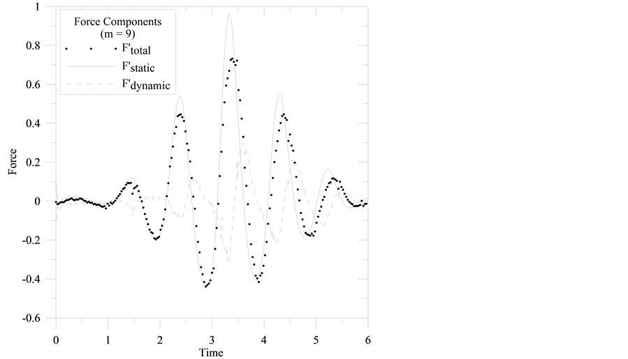
Figure 16. Non-dimensionalised force components for m = 9: max- mum excursion negative.
For the simulation of the mechanical system in CFD it is necessary to know the relationship between the two accelerated bodies, i.e. the float and the counter weight. The reason for this is that the CFD codes do not model the pulley system and the counter weight directly, and so these are approximated using additional body forces. The free body diagram as seen in Figure 19 is used to find the unknown tension forces in the cable T1 and T2 and the acceleration of the system.

Figure 17. Non-dimensionalised force components for m = 6: maxi- mum excursion positive.

Figure 18. Geometry.

Figure 19. Force analysis.
For the left hand side of system, representing the float, the force equilibrium is achieved when
 (41)
(41)
with mf being the mass of the float, the positive upward acceleration of the system, g is gravity, T1 represents the tension force in the cable and Fb is the buoyancy force. For the counterweight on the left hand side, the positive z-direction is downward, denoted z2, and the force equilibrium can be written as
 (42)
(42)
where mc is the mass of the counterweight and T2 the tension force in the cable. When moving the float vertically by a distance of z1 the counterweight covers the same distance, from which follows that  . Furthermore, the relationship between the tension forces can be written as.
The two unknowns of the system; the acceleration of the float and the tension force T, can then be written as
 (43)
(43)
and
 (44)
(44)
In the computational approach Fb is calculated from the integrated pressures on the float surface and thereby known at any time. The simulations are run using AMAZON and the FV solver with two alternative approaches to representing the effect of the float, pulley and counterweight arrangement. These are identified as case A and B and are defined in Table 4, in which the mass of the float and the applied tension force relating to Figure 19 are given.
For the numerical simulations NewWave focusing is used to generate the extreme wave [43] The concept of wave focusing is to generate several waves of relatively small amplitudes and different periods. These waves interact and constructive interfere to build up a localised extreme wave, larger than any individual wave created at the paddle, focussed at a specified position and time in the tank. For each wave component n the amplitude an is defined as
 (45)
(45)
where Sn(f) is the spectral density, Δf is the frequency step depending on the number of wave components and bandwidth and A is the target linear amplitude of the focussed wave. Thus, the amplitude of every spectral component in the NewWave group scales as the power density within that frequency band in the assumed sea-state. Equivalently, NewWave is simply the scaled auto-correlation function corresponding to a specified frequency spectrum such as the one obtained on the measured surface elevation time history at the location of the float without the float being in place during the physical tank tests.
The waves are generated using a velocity inlet at the left hand boundary of the numerical wave tank (NWT) at x = 0. Here, the surface elevation of the wave group is prescribed using the same techniques as described for the regular waves in Section 3.1 by specifying the vertical location of the water volume fraction of 0.5. The horizontal and vertical velocity components derived from NewWave theory are applied at the inlet boundary, such that t0 and x0 are the chosen focus time and location in the tank, here set to 4.6 s and 3.5 m respectively. N is the number of wave components, here 15. The numerically reproduced wave without the float in place using AMAZON and the FV solver can be seen in Figure 20 together with the measured elevation. Both numerical codes reproduce the focussed wave well. The FV solver predicts the asymmetry of the peak and trough values either side of the main peak particularly well, and the double peak evident in the experiment at the preceding peak is also predicted with this method. However, the depth of the preceding trough is slightly over predicted and there are some unphysical oscillations in the time history predicted for the first three seconds of the simulation. The AMAZON code predicts the peak of the main wave well, but there is a time lag in the prediction of the following wave and some differences in the position of the preceding wave. Details of the CPU run time and

Figure 20. Surface elevations at location of float without the float being in place.
computer architecture used by each of the codes for this case are summarized in Table 5.
Figures 21 (Case A) and 22 (Case B) show the comparison of predicted and measured vertical translation of the float as it interacts with the extreme wave. The set-up, including details of the mesh and the applied forces as well as an example of the NWT showing the free surface at a point in time as the focused wave approaches the float are shown in Figure 23 and in Figure 24 photographs of the experiment in the wave tank at Manchester University are given to show the large horizontal motions observed in addition to vertical motion of the float. It should be noted that these numerical simulations are restricted to vertical motion only and are therefore restrained in horizontal motion and rotation. This is a current limitation of the software and would explain the differences between the predicted and measured vertical motion of the float.
Case A, in which a constant tension force of T = mcg and the mass of float, mf ‒ mc are applied, predicts significant damping of the vertical motion response after the focused wave has passed although the initial motion of the float is predicted well. In case B, the tension force varies with the acceleration of the float calculated within the solution as, with the mass of float, mf. This leads to a much better prediction of the vertical motion in general, and whereas the response is slightly over-predicted as the extreme wave interacts with the float, its response is much better predicted following the extreme event. Thus the solution is much improved when the tension force includes the instantaneous acceleration of the float rather that assuming it is constant as in case A.
In case C, another Bobber shape is tested in the wave tank at Manchester University. In this test, the geometry of the Bobber is a flat-bottomed cylinder of radius 0.074 m with a corner radius of 0.033 m. The vertical sides extend to 0.085 m above the flat base and a conical upper surface with a 30 degree base angle decreases the radius of the geometry to 0.025 m at the upper cylindrical section (see Figure 25). Figure 26 shows the surface mesh of the flat-base Bobber. The outer dimensions of the numerical domain are and the water depth is 0.35 m. Two different particle densities are used and results presented in Figures 26 and 27. The number of particles in the coarse mesh is 118,000 with particle spacing of 0.04 m and the fine mesh is 918,000 with particle spacing of 0.02 m.
According to the experimental tests by Stallard et al. [41] and Weller et al. [41] , the float mass mf = 2.1 kg and the counterweight mass mc = 1.0 kg in case C. Figure 27 and Figure 28 show the comparison of SPH results and experimental data for the device response, using uniform particle mass and solving the dynamics in one and six degrees of freedom using two particle resolutions (Δx = 0.04 m and Δx = 0.02 m). The maximum
Table 4. Properties of manchester bobber cases.
Table 5. Details of the NWT used by each code for the manchester bobber case.
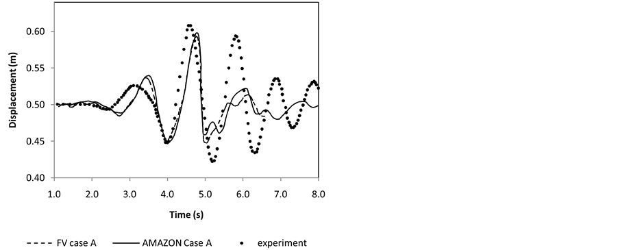
Figure 21. Translation of float (case A).
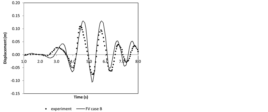
Figure 22. Translation of float (case B).
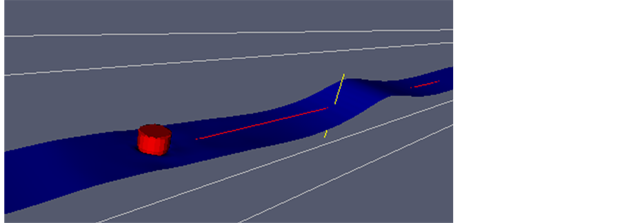

Figure 23. Details of the mesh and free surface at a point in time as the focused wave approaches the float.
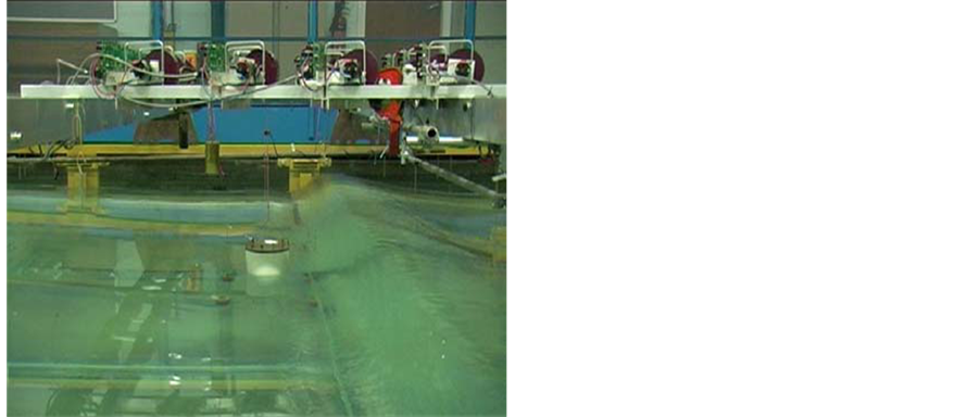
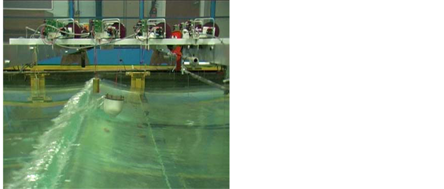
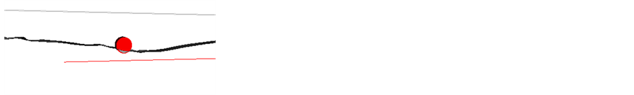
Figure 24. Position of the float in the physical experiments for two instances in time. Left: approaching large wave from the right. Right: the breaking wave has just passed the float, which is airborne. Counterweight and float have moved signi- ficantly from the position shown on the left.
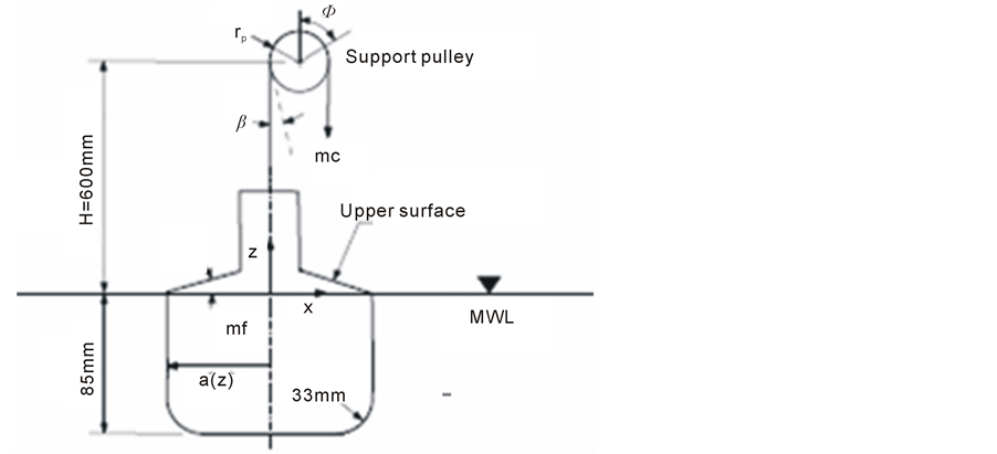
Figure 25. Case C geometry.

Figure 26. Case C bobber with flat-bottom cylinder.

Figure 27. Comparison of SPH result and experimental data for the device response using uniform particle mass, (Δx = 0.04 m), case C.

Figure 28. Comparison of SPH result and experimental data for the device response using uniform particle mass, (Δx = 0.02 m), case C.
wave amplitude produces the second peak in the device-response profile at t = 4.6 s or t/Tp = 3.2. The results are in agreement in terms of phase and magnitude. However, the SPH result for the coarse simulations seems to be oscillatory because the number of fluid particles interacting with the device is small, whereas for the finer resolution the response is considerably smoother and all the peaks are reproduced by the SPH results. In order to achieve a smoothed profile of device response, the number of fluid particles around the device needs to be considerably greater. Clearly, the SPH results for the system with six degrees of freedom are smoother and in better agreement (Figure 28 ) than the system with one degree of freedom.
4. Discussion and Conclusions
Three non-linear wave-structure interaction cases have been modelled using state-of-the-art CFD techniques that include three mesh-based techniques solving the Euler and Navier-Stokes equations, and one particle method. The cases increase in complexity, starting with a fixed horizontal cylinder in regular waves. The second case involves rigid vertical motion of a cone, which is forced to oscillate and radiate waves at the surface in still water. The last experiment shows the ability of the CFD methods to cope with highly non-linear wave and floating body interaction. Furthermore, in the last test the body not only interacted with waves, which was modelled sufficiently for smaller waves by Hadzic et al. [4] , but also with an attached mass, which is represented in the numerical simulations here by a body force.
The use of CFD for wave-structure interaction is usually only considered for situations in which assumptions such as inviscid and irrotational flow, linear wave theory and small body motion do not apply. In these situations, the detailed information provided through CFD modelling is of interest and must be considered alongside the accuracy of the results given by CFD, the computational costs and the flexibility in setup and problem definition. Generally the accuracy of the results increases with the number of cells/particles in the domain, and it is possible to capture highly non-linear effects like spray at the cost of larger run-times. Here, fluid forces, surface elevations and motions are predicted and compared with experimental data. For a fixed structure, the forces are well resolved by all methods applied and non-linear surface interaction was also captured successfully.
Body motion has been modelled in two ways. First, a cone-shaped body was forced at the free surface to radiate waves. The difficulties of this case for the mesh methods lay in the presentation of the body and its small maximum displacement. For free surface flow, the mesh should normally use hexahedral cells, as stated in Westphalen et al. [39] . However, for modelling the axisymmetric cone this is not beneficial, as either the cells are distorted (when using a body fitted grid) or arbitrarily shaped, which both introduce numerical errors. These increase when the mesh moves according to rigid body motion. In SPH this problem is non-existent. All results, however, showed good agreement.
The second case involving rigid body motion is the heave response of a floating body to interaction with an extreme focussed wave. Here, the results for the CFD packages differ. While the Navier-Stokes/FV solver computed the translation of the body with good agreement when the tension force was modelled by the gravitational component only, it overestimates the motion of the float when the tension force also includes the time-varying body acceleration. The problem of overestimation of the motion due to using the unsteady part of the tension force, needs to be resolved, and may well be due to the numerical solutions being limited to heave motion, whereas the experiments clearly show large surge motions as seen in Figure 24. The SPH certainly show better agreement with experiment with 6 degrees of freedom than with heave alone.
The extreme wave loading presented in this paper makes use of a NewWave design wave to reduce the run times. In reality, irregular waves excite the body continuously and these long-term irregular waves are needed to model the final device with mooring and PTO. The computational cost for such runs would increase significantly, not only for running the simulations but also for storing the results. The parallel capability of all the CFD packages used for this work makes it possible to reduce the wall clock time significantly, and in some cases symmetry can be employed to achieve further reductions. As the simulations presented here were performed on different platforms, direct comparisons are difficult. To give an example for the Navier-Stokes FV solver: The final simulation of 8 s of the floating body needed 5 days on 8 partitions using a desktop workstation (16 GB RAM, 2.5 GHz). The same simulation on a cluster took 3 days (2.5 GHz, 2 GB per node, Infiniband).
In this paper the use of CFD for wave loading on WECs is considered using four different CFD techniques. From the results presented it can be concluded that CFD is a versatile tool, capable of solving highly complex and non-linear wave-structure interaction problems. Each of the CFD methods considered predicted the wave structure interaction well and in generally good agreement with experimental results. The jet flow developed in the oscillating cone case is challenging for the Eulerian mesh based approaches as the resolution of the jet is limited by the grid size, and SPH is not limited in the same way and is better able to capture the jet.
Acknowledgements
The authors would like to acknowledge the support of the Engineering and Physical Sciences Research Councilfunded under the project title “Extreme Wave Loading on Offshore Wave Energy Devices using CFD: a Hierarchical Team Approach” (Grant No. EP/D077508).
Furthermore, many thanks go to Dr. Kevin Drake of University College London (UCL) for providing the high quality physical test data used for the cone simulations.
References
- WAMIT Inc. (2006) User Manual, Versions 6.4, 6.4 PC, 6.3, 6.3S-PC.
- Delhommeau, G. (1993) Seakeeping Codes AQUADYN and AQUAPLUS. In: Proceedings of the 19th WEGEMT SCHOOL on Numerical Simulation of Hydrodynamics: Ships and Offshore Structures, Nantes.
- Cummins, W.E. (1962) The Impulse Response Function and Ship Motions. Schiffstechnik, 47, 101-109.
- Hadzic, I., Hennig, J., Peric, M. and Xing-Kaeding, Y. (2005) Computation of Flow-Induced Motion of Floating Bodies. Applied Mathematical Modelling, 29, 1196-1210. http://dx.doi.org/10.1016/j.apm.2005.02.014
- Dixon, A.G., Greated, C.A. and Salter, S.H. (1979) Wave Forces on Partially Submerged Cylinders. Journal of the Waterway, Port, Coastal and Ocean Devision, 105, 421-438.
- Drake, K.R., Eatock Taylor, R., Taylor, P.H. and Bai, W. (2008) On the Hydrodynamics of Bobbing Cones. Ocean Engineering, 36, 1270-1277. http://dx.doi.org/10.1016/j.oceaneng.2009.07.007
- CD-Adapco (2009) STAR CCM+Version 4.04.011. London.
- Tu, J., Yeoh, G. and Liu, C. (2008) Computational Fluid Dynamics: A Practical Approach. 2nd Edition, Butter- worth-Heinemann, Oxford.
- Patankar, S.V. (1980) Numerical Heat Transfer and Fluid Flow. Taylor & Francis, London.
- Patankar, S.V. and Spalding, D.B. (1972) A Calculation Procedure for Heat, Mass and Momentum Tranfer in Three- Dimensional Parabolic Flows. International Journal of Heat and Mass Transfer, 15, 1787-1806. http://dx.doi.org/10.1016/0017-9310(72)90054-3
- Hirt, C.W. and Nichols, B.D. (1981) Volume of Fluid (VOF) Method for the Dynamics of Free Boundaries. Journal of Computational Physics, 39, 201-225. http://dx.doi.org/10.1016/0021-9991(81)90145-5
- Ubbink, O. (1997) Numerical Prediction of Two Fluid Systems with Sharp Interfaces. PhD: 138, Department of Me- chanical Engineering, Imperial College of Science, Technology & Medicine, London.
- Greaves, D.M. (2004) A Quadtree Adaptive Method for Simulating Fluid Flows with Moving Interfaces. Journal of Computational Physics, 194, 35-56. http://dx.doi.org/10.1016/j.jcp.2003.08.018
- Ferziger, J.H. and Peric, M. (2001) Computational Methods for Fluid Dynamics. Springer, Heidelberg.
- Ansys, I. (2006) ANSYS CFX-Solver Theory Guide. Canonsburg. http://www.ansys.com/staticassets/ANSYS/staticassets/resourcelibrary/brochure/ansys-cfx-tech-specs.pdf
- Baliga, B.R. and Patankar, S.V. (1980) A New Finite-Element Formulation for Convection-Diffusion Problems. Nu- merical Heat Transfer, Part A, 3, 393-409.
- Baliga, B.R. and Patankar, S.V. (1983) A Control Volume Finite-Element Method for Two-Dimensional Fluid Flow and Heat Transfer. Numerical Heat Transfer, Part A, 6, 245-261.
- Barth, J.T. and Jesperson, D.C. (1989) The Design and Application of Upwind Schemes on Unstructured Meshes. American Institute of Aeronautics and Astronautics (AIAA), Reno.
- Zwart, P.J., Scheuerer, M. and Bogner, M. (2003) Free Surface Modelling of an Impinging Jet. ASTAR International Workshop on Advanced Numerical Methods for Multidimensional Simulation of Two-Phase Flow, Garching, 15-16 September 2003.
- Zwart, P.J. (2005) Numerical Modelling of Free Surface and Cavitating Flows. VKI Lucture Series, Ansys Canada Ltd, Canada, 25.
- Rhie, C.M. and Chow, W.L. (1982) A Numerical Study of the Turbulent Flow Past an Isolated Airfoil with Trailing Edge Separation. AIAA/ASME 3rd Joint Thermophysics, Fluids, Plasma and Heat Transfer Conference, St. Louis, 7-11 June 1982. http://dx.doi.org/10.2514/6.1982-998
- Monaghan, J.J. (2005) Smoothed Particle Hydrodynamics. Reports on Progress in Physics, 68, 1703-1759. http://dx.doi.org/10.1088/0034-4885/68/8/R01
- Vila, J.P. (1999) On Particle Weighted Methods and Smoothed Particle Hydrodynamics. Mathematical Models and Methods in Applied Sciences, 9, 161-209.
- Guilcher, P.M., Ducorzet, G., Alessandrini, B. and Ferrant, P. (2007) Water Wave Propagation Using SPH Models. Proceedings of 2nd International SPHERIC Workshop, Madrid, 23-25 May 2007, 119-124.
- Toro, F. (2001) Shock-Capturing Methods for Free-Surface Shallow Flows. John Wiley & Sons LTD, Hoboken.
- Hirsch, C. (1990) Numerical Computation of Internal and External Flows, volume 2: Computational Methods for In- viscid and Viscous Flows, Wiley, Hoboken.
- Chatkravathy, S.R. and Osher, S. (1983) High Resolution Applications of the Osher Upwind Scheme for the Euler Equations, AIAA Paper 83-1943. Proceedings of AIAA 6th Comutational Fluid Dynamics Conference, Danvers, July 1983, 363-373.
- SPHysics. (2010) HYPERLINK. http://wiki.manchester.ac.uk/sphysics.
- Monaghan, J.J. and Kos, A. (1999) Solitary Waves on a Creatan Beach. Journal of Waterway, Port, Coastal and Ocean Engineering, 125, 145-154. http://dx.doi.org/10.1061/(ASCE)0733-950X(1999)125:3(145)
- Chorin, A.J. (1968) Numerical Solution of the Navier-Stokes Equations. Mathematics of Computation, 22, 745-762.
- Cummins, S.J. and Rudman, M. (1999) An SPH Projection Method. Journal of Computational Physics, 152, 584-607.
- Lind, S., Xu, R., Stansby, P. and Rogers, B. (2012) Incompressible Smoothed Particle Hydrodynamics for Free-Surface Flows: A Generalised Diffusion-Based Algorithm for Stability and Validations for Impulsive Flows and Propagating Waves. Journal of Computational Physics, 231, 1499-1523. http://dx.doi.org/10.1016/j.jcp.2011.10.027
- Skillen, A., Lind, S., Stansby, P. and Rogers, B. (2013) Incompressible Smoothed Particle Hydrodynamics (SPH) with Reduced Temporal Noise and Generalised Fickian Smoothing Applied to Body-Water Slam and Efficient Wave-Body Interaction. Computer Methods in Applied Mechanics and Engineering, 265, 163-173. http://dx.doi.org/10.1016/j.cma.2013.05.017
- Xu, R., Stansby, P.K. and Laurence, D. (2009) Accuracy and Stability in Incompressible SPH (ISPH) Based on the Projection Method and a New Approach. Journal of Computational Physics, 228, 6703-6725. http://dx.doi.org/10.1016/j.jcp.2009.05.032
- Qian, L., Causon, D.M., Mingham, C.G. and Ingram, D.M. (2006) A Free Surface Capturing Method for Two Fluid Flows with Moving Bodies. Proceedings of the Royal Society A: Mathematical, Physical and Engineering Science, 462, 21-42.
- Causon, D.M., Ingram, D.M., Mingham, C.G., Yang, G. and Pearson, R.V. (2000) Calculation of Shallow Water Flows Using a Cartesian Cut Cell Approach. Advances in Water Resources, 23, 545-562. http://dx.doi.org/10.1016/S0309-1708(99)00036-6
- Causon, D.M., Ingram, D.M. and Mingham, C.G. (2001) A Cartesian Cut Cell Method for Shallow Water Flows with Moving Boundaries. Advances in Water Resources, 24, 899-911. http://dx.doi.org/10.1016/S0309-1708(01)00010-0
- Westphalen, J. (2010) Extreme Wave Loading on Offshore Wave Energy Devices Using CFD. PhD Thesis, University of Plymouth, Plymouth, 73-75.
- Westphalen, J., Greaves, D., Williams, C.J.K., Zang, J. and Taylor, P. (2008) Numerical Simulation of Extreme Free Surface Waves. Proceedings of the 18th International Offshore and Polar Engineering Conference, Vancouver, 6-11 July 2008.
- Rogers, B.D. and Dalrymple, R.A. (2008) SPH Modelling of Tsunami Waves. In: Advances in Coastal and Ocean Engineering Vol. 10, Advanced Numerical Models for Tsunami Waves and Runup. W. Scientific, Singapore.
- Stallard, T., Weller, S.D. and Stansby, P.K. (2009) Limiting Heave Response of a Wave Energy Device by Draft Ad- justment with Upper Surface Immersion. Applied Ocean Research, 31, 282-289. http://dx.doi.org/10.1016/j.apor.2009.08.001
- Weller, S.D., Stallard, T.J. and Stansby, P.K. (2012) Experimental Measurements of the Complex Motion of a Sus- pended Axisymmetric Floating Body in Regular and Near-Focused Waves. Applied Ocean Research, 39, 137-145.
- Taylor, P.H. and Williams, B.A. (2004) Wave Statistics for Intermediate Depth Water-NewWaves and Symmetry. Journal of Offshore Mechanics and Arctic Engineering, 126, 54-59. http://dx.doi.org/10.1115/1.1641796
Nomenclature
A = Wave amplitude or maximum excursion
A' = Relative amplitude
An = Amplitude of each wave component
B = Body force
c = Volume fraction (the water surface of the c = 0.5) or crest focussed
d = Displacement
d' = Relative axis depth
d(t) = Displacement of motion of the cone
D = Diameter of cylinder
F = Force
F = Flux vector function
F' = Non-dimensionalised force
Fb = Buoyancy force
Fz = Vertical force
G = Acceleration duo to gravity
H = Water level
K = Wave number
kA = Wave steepness
l = Length of cylinder
m = Integer
mc = Mass of the counterweight
mf = Mass of the float
n = Normal vector
N = Number of frequency components
KC = Keulegan-Carpenter number
P = Pressure
R = Radius of cone at still water level
S = Source term
Sb = Body surface
Sn(f) = Spectral density
T = Time
t0 = Focussed time
T = Wave period, Trough focussed or tension force
T1, T2 = Tension force in the cable
U = Velocity vector
u,v,w = Components of u
V = Domain of interest
X = Position vector
x,y,z = Coordinate directions
z1 = Positive upward z distance
z2 = Positive downward z direction
 = Positive upward acceleration
 = Positive downward acceleration
Δωn = Central circular frequency step
Δf = Frequency step
Δx = Particle resolution
ɳ = Surface elevation
ω = Frequency
ω0 = Central circular frequency
ρ = Density
f = General flow property