Open Journal of Fluid Dynamics
Vol.3 No.1(2013), Article ID:29376,9 pages DOI:10.4236/ojfd.2013.31003
Analysis on Physical Mechanism of Sound Generation inside Cavities Based on Acoustic Analogy Method
1State Key Laboratory of Aerodynamics, China Aerodynamics Research and Development Center, Mianyang, China
2High Speed Aerodynamics Research Institute, China Aerodynamics Research and Development Center, Mianyang, China
3School of Aerospace, Tsinghua University, Beijing, China
Email: yangdg-cardc@163.com
Received September 2, 2012; revised October 13, 2012; accepted October 25, 2012
Keywords: Cavity; Physical Mechanism; Sound Generation; Aerodynamic Noise; Sound Pressure Level; Sound Pressure Frequency Spectrum
ABSTRACT
Analysis of coupling aerodynamics and acoustics are performed to investigate the self-sustained oscillation and aerodynamic noise in two-dimensional flow past a cavity with length to depth ratio of 2 at subsonic speeds. The large eddy simulation (LES) equations and integral formulation of Ffowcs-Williams and Hawings (FW-H) are solved for the cavity with same conditions as experiments. The obtained density-field agrees well with Krishnamurty’s experimental schlieren photograph, which simulates flow-field distributions and the direction of sound wave radiation. The simulated self-sustained oscillation modes inside the cavity agree with Rossiter’s and Heller’s predicated results, which indicate frequency characteristics are obtained. Moreover, the results indicate that the feedback mechanism that new sheddingvortexes induced by propagation of sound wave created by the impingement of the shedding-vortexes in the shear-layer and rear cavity face leads to self-sustained oscillation and high noise inside the cavity. The peak acoustic pressure occurs in the first oscillation mode and the most of sound energy focuses on the low-frequency region.
1. Introduction
High-speed compressible flows past open cavities induce complex unsteady aerodynamic characteristics, such as flow separation in the cavity front-face, shear-layer instabilities, vortex shedding, shock waves/boundary-layer interactions and self-sustained flow oscillations within the cavity. Under certain conditions, the strong self-sustained flow oscillations associated with large-amplitude noises around 150 dB for high-speed flows can occur in a flow past an open cavity [1]. This phenomenon is thought to arise from a complex feedback mechanism involving the amplification and convection of small instabilities by the shear layer, whose impingement at the downstream corner generates acoustic waves. In turn, these acoustic waves travel upstream and excite further disturbances in the shear layer, leading to a new selfsustained oscillation process [2]. The severe noise environment can represent a potential hazard to structure security of the cavity apparatuses inside the cavity.
Oscillation in the flow past an open cavity has been investigated for decades, still there remain many open questions about even the basic physical mechanisms underlying the self-sustained oscillations. Cavity oscillations in compressible flows are typically described as a flow-acoustic resonance phenomenon, and its first detailed description is credited to Rossiter (1964) who proposed a semiempirical formula for predicting the frequency peaks in high subsonic compressible flows over shallow cavities, named open cavities, with a length-todepth ratio  [3]. In this mechanism, small disturbances in the free-stream shear layer spanning the cavity are amplified via Kelvin Helmholtz instability. Their interaction with the trailing cavity edge gives rise to an unsteady flow-field, the upstream influence of which excites further disturbances to the free-stream shear layer, especially near the cavity leading edge [4]. In 1975, Heller modified the formula who presented the radiation velocity of feedback acoustic waves from the cavity rear-face to front-face should be the local velocity of sound [5]. Another analysis mode of cavity oscillation was obtained in the early work by Bilanin [6] and Tam [7], and the mode, in some sense, can predict peak frequencies of cavity tones but no sound pressure magnitude.
Nowadays, numerical simulation investigations have been performed for cavity oscillations and aeroacoustic characteristics based on the development in CFD technique. Previous numerical studies of compressible cavity flows have used the two dimensional unsteady RANS (Reynolds averaged Navier-Stokes) equations with a k-w turbulence model (Lamp & Chokani 1997; Zhang, Rona & Edwards 1998; Fuglsange & Cain 1992). The effectiveness of compressible turbulence models for separated oscillating flows, and especially their radiated acoustic field (which, as noted above, is an integral part of the resonant instability modes) remains an open question. Direct numerical simulation (DNS) is an accurate numerical method to simulate turbulence, but it requires high cost and computational capacities. Fortunately, Large Eddy Simulations (LES) provide a means to study the details of the modes of oscillation and the basic physical mechanisms of sound generation [8,9]. Computational Aero-Acoustics (CAA) also presents some advantages in studies on aeroacoustic characteristics of cavity flow.
The purpose of the study is to indicate the self-sustained oscillations and the physical mechanisms of sound generation inside an open cavity. The numerical simulation method is to analyze the unsteady flow characteristics in the near flow-flied by utilizing LES, and to predict sound radiation and acoustic-flied by solving Ffowcs Williams-Hawking (FW-H) equations [10].
2. Flow Calculation Methods
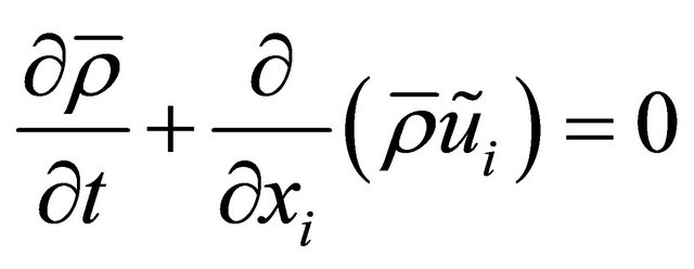
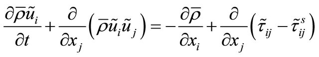
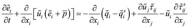
A LES model was initially employed to run the two dimensional cavity flow simulations. The numerical model is a compressible flow LES model. In Cartesian coordinates, the box-filtered equations are utilized to obtain the equations [11,12] , shown as follows,
 (1)
(1)
 (2)
(2)
 (3)
(3)
where symbols overbar, tilde and superscripts denote Reynolds, box-filtered quantities and sub-grid scale quantities respectively.  are density, velocity components, pressure, temperature, total energy, viscous stress tensor and sub-grid stress tensor, respectively. There are auxiliary relations,
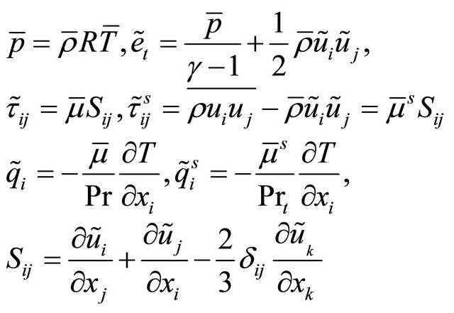
where constants , The molecular viscosity
  and eddy viscosity
  is modeled by sub-grid (SGS) models. In a mixedscale SGS model [13],
 (4)
(4)
 (5)
(5)
 (6)
(6)
where
Advantages of mixed-scale model are no artificial averaging and wall-damping function required. A 2nd order central finite-difference scheme is employed for the spatial discretization [14,15]. The time integration scheme is a 3rd order Runge-Kutta scheme [16,17]. By placing a buffer-zone combined together with Giles characteristic condition as a non-reflecting boundary condition (NRC) in inflow and outflow regions this code performs better than without buffer zone conditions [18].
3. Acoustic Wave Propagation
Finally, complete content and organizational editing before formatting. Please take note of the following items when proofreading spelling and grammar: Ffowcs Williams and Hawkings derived the most general form of wave equation using the technique of generalized function theory which allowed them to utilize the free-space Green function in constructing the integral solution. The aeroacoustic prediction method is presented in reference [19]. An advanced time method for aeroacoustic predictions has been proposed recently [20]. For the same FW-H formulation developed by Farassat and Succi [21], it has a different implementation compared with a traditional retarded time method [21]. The basic idea is that at a far field observer, acoustic signals emitted from each panel of an integration surface are predicted through an FW-H solver and are gathered at different observer time levels. For an observer at a certain time only part of the sound pressure contribution is received. A sound pressure prediction will be completed when all signals from the integration surface are received. Far field directivity is calculated at a final stage. As a result of [20], the FW-H solver can now be integrated in the CFD solver and works in a parallel computing environment to provide a far field acoustic pressure prediction in line with the CFD near field prediction. This method does not require hard disk storage and hence is called a low storage FW-H solver. The low storage FW-H solver is essential for far field aeroacoustic predictions in 3-D turbulent flow simulations since usage of hard disk storage would be excessive with previous approaches.
According to reference [19], sound pressure consists of thickness noise , loading noise
  and quadruple noise
 ,
,
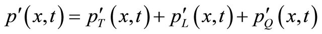 (7)
(7)
where,
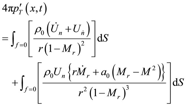 (8)
(8)
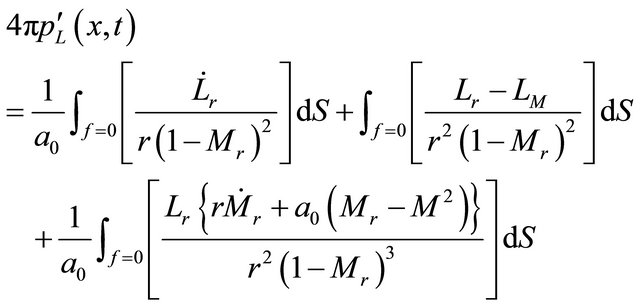 (9)
(9)
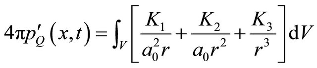 (10)
(10)
Details of those parameters can be found in reference [22]. Note that the quadrupole noise  is not included in this solver. Values of the quadrupole noise
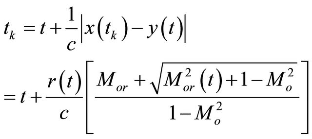
  are small as long as the integration surface is placed away from the strong flow non-linear interaction region (source region), such as free shear layer and viscous boundary layer. Equations (8) to (10) are similar to the retarded time formulations except that the surface integral is dropped since the formulation is for an individual panel while in the retarded time method it is for all panels. The advanced time is the time at which a disturbance emitted by a source element y at time t will reach the observer x. For a subsonic observer velocity it is,
 (11)
(11)
It is often the case that the flow is computed with a two-dimensional cavity model, such as reference [4] (Rowley, et al., 2002) and reference [23] (Sung-Eun Kim, et al., 2003). For two-dimensional CFD models on which the FH-W integrals are to be evaluated, the current implementation allows users to specify what can be called a “correlation-length ” over which the flow is assumed to be perfectly correlated. The correlation-length is used as an effective length when the FW-H’s surface integrals are evaluated [22].
4. Acoustic Parameters
Some acoustic parameters analyzed are sound pressure level (SPL), sound pressure frequency spectrum (SPFS) and Strouhal number (St). Herein SPL denotes pressure fluctuation magnitude, which was calculated by Equation (12). SPFS denotes sound pressure spectral energy on the different discrete frequencies, which was calculated by Equation (13). St calculated by Equation (14) is a nondimensional number which denotes oscillation frequency inside cavities.  is the sound pressure spectral density function, which was calculated by FFT and defined by was Equation (15). Therein Prms is the rootmean-square of the pressure fluctuation, which was obtained by integrating the power spectral density in the frequency band of 0 - 10 kHz and extracting the square root. Pref is the benchmark sound pressure, 20 mPa. f denotes oscillation frequency, and L is the cavity length, and
  is free-stream velocity, and T is a special time to collect experimental data, and
  denotes frequency range to analyze SPFS characteristics.
 (12)
(12)
 (13)
(13)
 (14)
(14)
 (15)
(15)
5. Code Validations
A quintessential code validation example is the aerodynamic noise generated by turbulent flow past a circular cylinder. Predicting the noise radiated from this seemingly simple configuration is not an easy task, mainly due to the difficulty of obtaining an accurate prediction of the flow when it is turbulent. We took here the case experimentally investigated by Revell et al. [24], which was also studied by others as a benchmark problem at the second Computational Aeroacoustics Workshop on Benchmark Problems. The diameter of the cylinder  is 0.019 m, and the free-stream velocity of the airflow
  is such that the Reynolds number (ReD) and Mach number (Ma) are 90,000 and 0.2, respectively. Brentner et al. computed the flow and noise for the same case using the FW-H approach and the near-field flow obtained from URANS predictions. In the present work, the flow was computed by LES with the Smagorinsky’s subgrid-scale viscosity model using a two-dimensional CFD model on a 100,000-cell quadrilateral mesh (See Figure 1). Although any earnest LES requires a threedimensional model, it was deemed that the two-dimensional model suffices to serve the objective of the present work. Besides, two-dimensional LES sheds much light on the actual three-dimensional flow, often being able to predict major flow features surprisingly well, as will be seen later.
According to reference [25], the time-step  of
of  was used for the transient simulation. The cylinder wall was used as the integration surface. Three different correlation lengths
  were tried in the acoustic calculations. The sound pressure signals were computed at two receiver locations: Receive-1 at 128D (2.432 m) and Receive-2 at 35D (0.665 m) away from the cylinder at 90˚ measured clockwise from the front stagnation point.
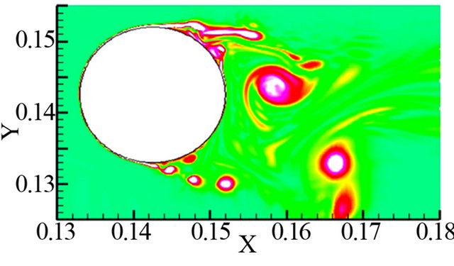
The contours of instantaneous vorticity at a different time instant (T is computational period) are depicted in Figure 2, and it can be seen that highlighting large scale structures in the wake indicative of an alternate vortexshedding, and smaller eddies near the separated shear layer from the cylinder also appear. Figures 3 and 4 show the time-history of lift  and drag coefficient (CD), respectively. Its time-averaged value CD) was found to be approximately 1.418 which is larger than the experimentally measured value of 1.320 [24] by about 10%, yet is remarkably better than the 2D-LES prediction presented by Sung-Eun Kim et al. (2003) [23] and the URANS predictions reported by Brentner et al.(1996) which all under predicted CD by 25% - 55%. The predicted Strouhal number
  also agrees quite better with the measured one
  than others. The predicted time-averaged drag coefficient and Strouhal number are summarized in Table 1.
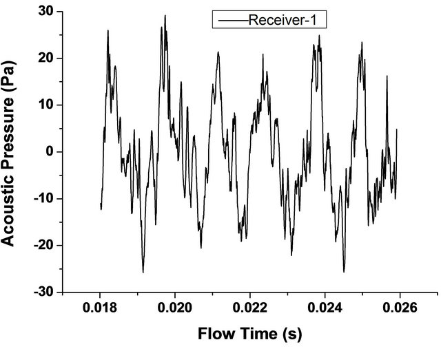
Figure 5 shows an instantaneous value at different flow time of the acoustic pressure signal at the receiver-1 and receiver-2 located 35D and 128D away from the cylinder at 90˚ measured clockwise from the front stagnation point computed using the correlation length of 5D
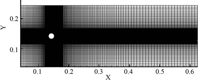
Figure 1. Computational domain and mesh.
 (a)
(a)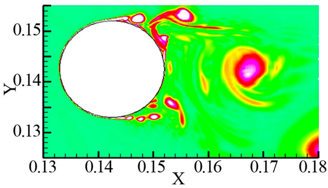 (b)
(b)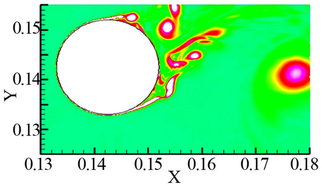 (c)
(c)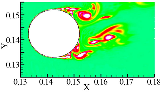 (d)
(d)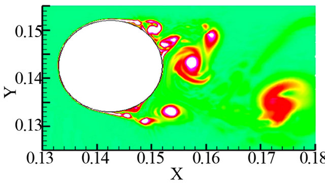 (e)
(e)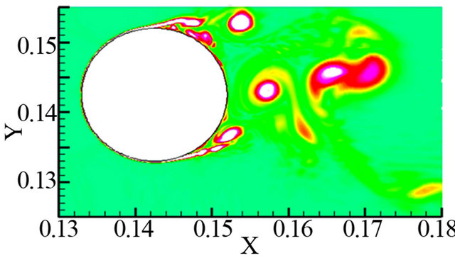 (f)
(f)
Figure 2. Close-up view of the contours of instantaneous vorticity around the circular cylinder (ReD = 90000). (a) 0T; (b) 0.25T; (c) 0.5T; (d) 0.75T; (e) 1T; (f) 1.25T.
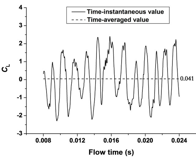
Figure 3. The time-history of lift coefficient.
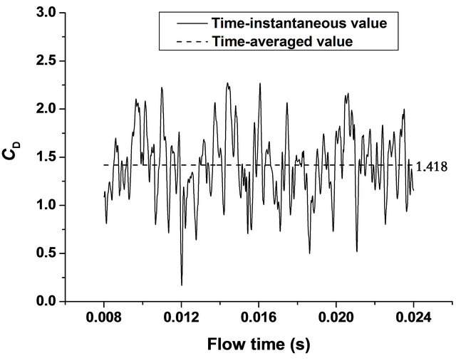
Figure 4. The time-history of drag coefficient.
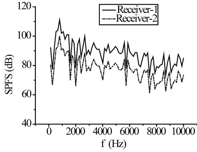
and the corresponding power spectral density, respectively. The aeroacoustic characteristics, SPFS and PSD, predicted at the two receivers are presented in Figure 6. The receiver-1 is nearer the cylinder wall of sound source, so the SPFS and PSD are higher than those at receiver-2 which can be seen from Figure 6. The aeroacoustic characterristics predicted are summarized in Table 2. These results presented in the paper are largely consistent with the results of Sung-Eun Kim et al. (2003) [23] and the experimental results obtained by Revell et al. (1977) [24]. Above analysis indicates that the numerical method utilized to compute sound in the paper is feasible.
Table 1. Averaged drag coefficient and Strouhal number predicted for the circular cylinder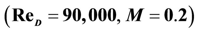 .
.
 (a)
(a) (b)
(b)
Figure 5. Acoustic pressure at the receivers located 35D and 128D away from the cylinder.
6. Cavity Model
The geometrical parameters of the cavity model in the paper are same as that researched by Rowley [4]. The computational conditions in numerical simulation are selected according to experimental parameters carried out by Krishnamurty et al. [25]. The computational domain and boundary conditions are shown in Figure 7, and the cavity length to depth ratio is 2, and the free-stream Mach number (Ma) is 0.64, and the Reynolds number is 1.16 × 10⁶ based on cavity length, and the sound signals are received on receiver-1 at the cavity front wall and receiver-2 at the cavity rear wall, respectively. It should be noted that the quoted values of the boundary-layer momentum thickness at the upstream cavity edge, are taken from the initial condition for each run. The oscillations that develop in the cavity can alter this value. The boundary-layer thickness to cavity depth ratio is 0.038. The computational domain is 300 thousand structure mesh, shown in Figure 8. In order to obtain
 (a)
(a)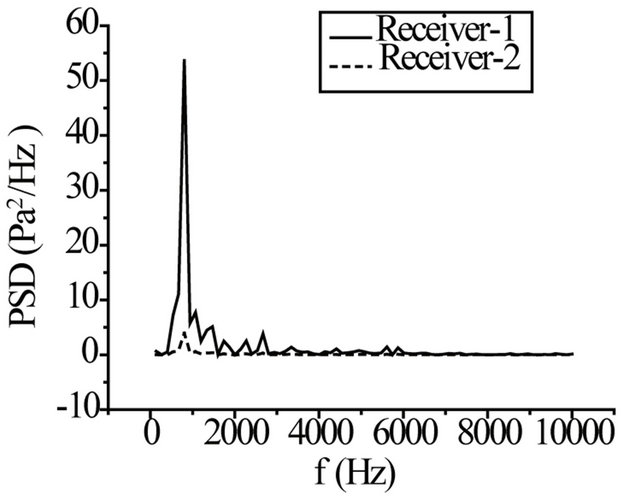 (b)
(b)
Figure 6. Aero-acoustics at receiver-1 and receiver-2. (a) Sound pressure frequency spectrum; (b) Sound pressure spectrum density.
Table 2. Aero-acoustic characteristics at receiver-point-1 and receiver-point-2.
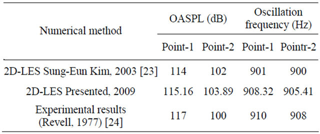
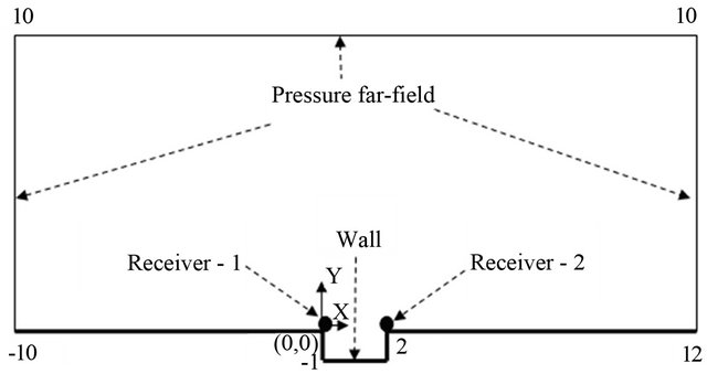
Figure 7. Computational domain and boundary conditions.
accurate sound source signal, the sound source correlation lengths  is selected to 5L for two-dimensional cavity model according to some references.
7. Self-Sustained Oscillation
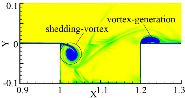
Figure 9 shows the developing process of instantaneous vorticity contours in the cavity flow-field in a flow period. High-speed flow past the cavity, vortex occurs near the front and rear walls of the cavity at 0.25T (T is numerical simulation period), shown in Figure 9(a) Flow
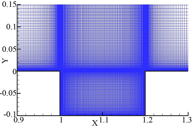
Figure 8. The computational mesh.
 (a)
(a)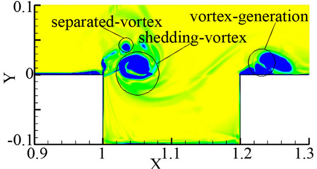 (b)
(b)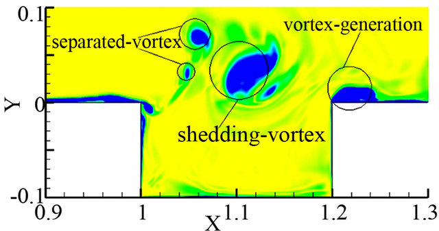 (c)
(c)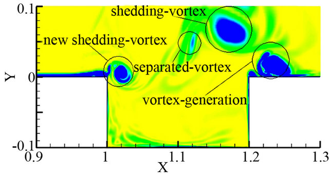 (d)
(d)
Figure 9. Instantaneous vorticity contours in the cavity Ⅰ. (a) 0.25T; (b) 0.5T; (c) 0.75T; (d) 1T.
separation appears and the vortex sheds and induces a new separated-vortex at the front wall of the cavity at 0.5T (see Figure 9(b)). At 0.75T, the shedding-vortex moves to the cavity rear wall, seen from Figure 9(c). After that, the shedding-vortex keeps on moving and a new shedding-vortex occurs near the cavity front wall at one period (see Figure 9(d)). Therefore, free-stream shear-layer separates at the cavity front edge, which induces vortex generation, development and shedding at some frequency over the cavity. Figure 10 illustrates instantaneous vorticity contours in the cavity flow-field at different flow time after 10 computational periods. At 0.25T, shedding-vortex and new generation vortex over
 (a)
(a)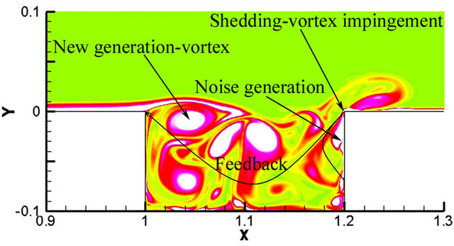 (b)
(b)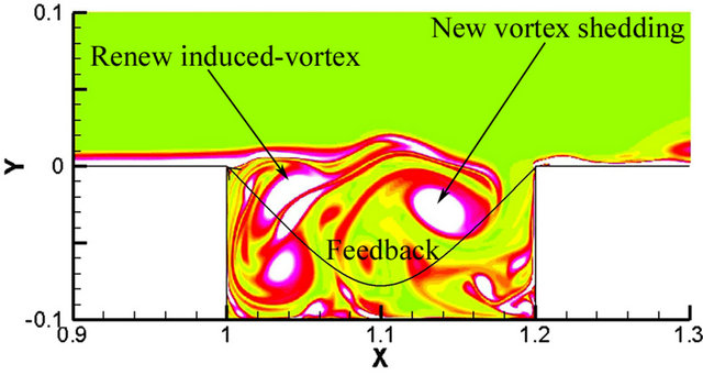 (c)
(c)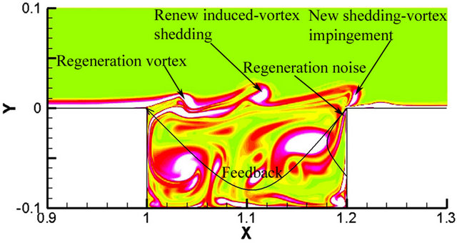 (d)
(d)
Figure 10. Instantaneous vorticity contours in the cavity Ⅱ. (a) 10.25T; (b) 10.5T; (c) 10.75T; (d) 11T.
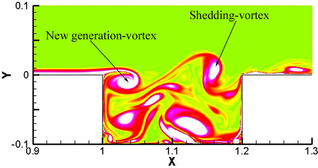
the cavity are induced by flow past the open cavity, shown in Figure 10(a). After 0.25T, the shedding-vortex impinges the cavity rear wall, and intense aerodynamic noise is induced by the impingement in the region near the cavity rear wall. The noise radiates from the cavity rear wall to the front region of the cavity, and the sound feedback occurs within the cavity. At the same time, the new generation vortex sheds and moves to the cavity rear wall (see Figure 10(b)). The sound feedback mechanism makes a renew induced-vortex generation at the cavity front wall (see Figure 10(c)). When the new generation vortex-shedding impinges the cavity rear wall again, and regeneration aerodynamic noise appears, and the sound feedback to the cavity front wall again induces regeneration vortex, shown in Figure 10(d). Therefore, a sound feedback mechanism and self-sustained flow oscillation of vortex generation, shedding-vortex, aerodynamic noise generation, vortex regeneration and re-shedding and aerodynamic noise regeneration within the open cavity.
8. Aeroacoustic Characteristics
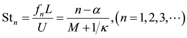
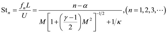
A set of non-dimensional modal peak oscillation frequencies within a open cavity at which acoustic tone amplitude occurs can be predicted by a Rossiter’s semiempirical Eqation (16) determined by Rossiter in 1964. Heller modified the equation in 1975 who presented radiate velocity of turbulence sound wave upward should be local sound velocity, and the modified equation is given as Equation (17).  is Strouhal number which indicates flow oscillation modes and peak frequencies of cavity acoustic tones.
  is n mode peak oscillation frequency, and U is free-stream velocity, and constant
  and
and . We performed a Fast Fourier Transform Algorithm (FFT) of 150 samples (every 300 time units) of the computational data over a period of time
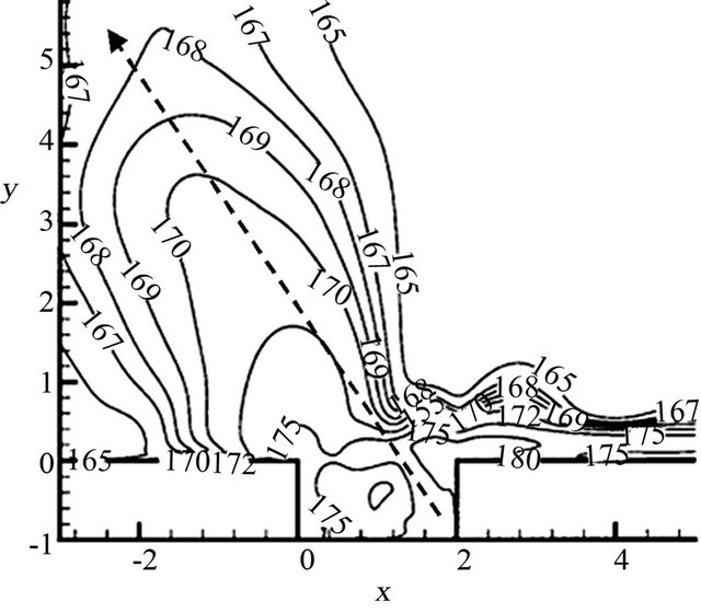
 , corresponding to 15 periods of the lower frequency, and 25 periods of the higher frequency. The resulting data record is approximately periodic in time, and any drift in the data is removed prior to taking the FFT. Figure 11 shows acoustic field predicted by Rowley, et al. (see Figure 11(a)) and presented in the paper (See Figure 11(b)). The results indicate that there is a very good qualitative agreement in between 2D-DNS and 2D-LES computational methods. The SPL distributions obtained by the two numerical simulation methods are similar, and the sound radiates to top left corner from the cavity at the Mach numbers.
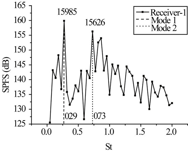
Figure 12 shows sound pressure frequency spectrum and power spectrum density at receiver-1 and receiver-2. Self-sustained oscillation mode 1 and mode 2, St1 and St2, within the cavity are about 0.29 and 0.73, respectively, which is similar with the results predicted by Rossiter and Heller (see Table 3). From pre-analysis, it can be known that aerodynamic noise is induced by vortex-
 (a)
(a)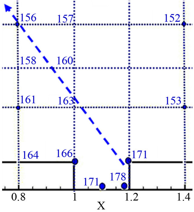 (b)
(b)
Figure 11. SPL distributions at measurement positions. (a) 2D-DNS (Rowley, et al. 2002); (b) 2D-LES (Presented, 2009).
Table 3. Analysis of self-sustained oscillation modes inside the cavity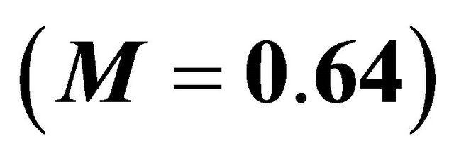 .
.
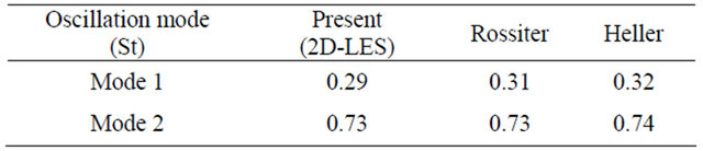
generation, development and shedding and impingement of the vortex and the cavity wall at subsonic speeds. The receiver-2 locates in a region near the cavity rear wall, aerodynamic noise generation appear in the region. Therefore, the SPFS at the self-sustained oscillation mode 1 of the receiver-2 is more than that of the receiver-1. For flow self-sustained oscillation characteristics inside the cavity, the mode 1 is a key self-sustained oscillation and on which peak frequency of cavity tone and sound pressure amplitude occurs, and the oscillation energy mostly focuses on mode 1.
 (16)
(16)
 (17)
(17)
 (a)
(a)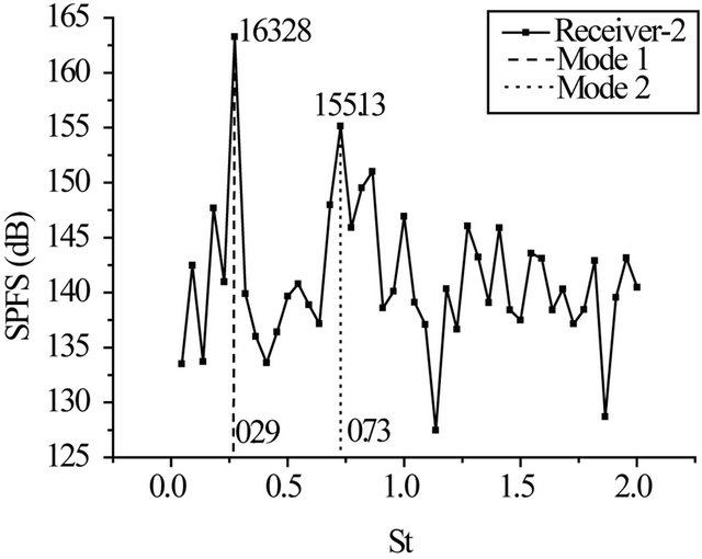 (b)
(b)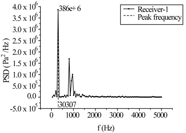 (c)
(c)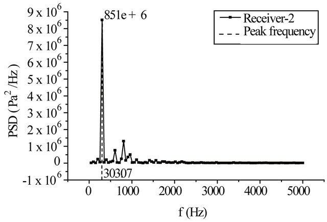 (d)
(d)
Figure 12. SPFS and PSD at two receivers. (a) SPFS of the receiver-1; (b) SPFS of the receiver-2; (c) PSD of the receiver-1; (d) PSD of the receiver-2.
9. Concluding Remarks
A study on physical mechanism of sound generation inside an open cavity with length to depth ratio  of 2 was conducted by numerical simulation method. There are the near field cavity CFD simulations by LES and the far field aero-acoustic predictions by FW-H integral equation. The results about the aerodynamic noise generated by turbulent flow past a two-dimensional circular cylinder indicate that a quintessential code validation is feasible. Acoustic energy focuses on self-sustained flow oscillation mode 1, and the oscillation mode predicted by the method is good agreement with Rossiter and Heller’s predicted results. The self-sustained flow oscillation and intense aerodynamic noise within the open cavity are induced by free-stream shear-layer separation, vortexgeneration-development-shedding, interaction of the shearlayer and flow within the cavity and impingement of flow and the cavity wall. Moreover, a sound feedback mechanism and self-sustained flow oscillation of vortex generation, shedding-vortex, aerodynamic noise generation, vortex regeneration and re-shedding and aerodynamic noise regeneration within the open cavity.
10. Acknowledgements
We should please to thank Pro Weimin JIANG in CARDC and Pro Cunbiao LI in Peking University for many helpful comments, and for suggesting the windtunnel test methodology and theoretical analysis. We should also thank High-speed Aerodynamics Institute of China Aerodynamics Research and Development Center for affording experimental apparatuses. The researched work was supported by Government fund “973” project (Number: 2009CB723802) and CARDC research fund.
REFERENCES
- N. Delprat, “Rossiter’s Formula: A Simple Spectral Model for a Complex Amplitude Modulation Process?” Physics of Fluids, Vol. 18, No. 7, 2006, Article ID: 071703. doi:10.1063/1.2219767
- D. Rockwell and E. Naudascher, “Review: Self-Sustaining Oscillations of Flow Past Cavities,” Journal of Fluids Engineering, Vol. 100, No. 2, 1978, pp. 152-165. doi:10.1115/1.3448624
- J. E. Rossiter, “Wind Tunnel Experiments of the Flow over Rectangular Cavities at Subsonic and Transonic Speeds,” ARCR & M, 1964, p. 3458.
- C. W. Rowley, T. Colonius and A. J. Basu, “On Self- Sustained Oscillations in Two-Dimensional Compressible Flow over Rectangular Cavities,” Journal of Fluid Mechanics, Vol. 455, 2002, pp. 315-346. doi:10.1017/S0022112001007534
- H. H. Heller and D. B. Bliss, “Aerodynamically Induced Pressure Oscillations in Cavities. Physical Mechanisms and Suppression Concepts,” Defense Technical Information Center, Fort Belvoir, 1975.
- A. J. Bilanin and E. E. Covert, “Estimation of Possible Excitation Frequencies for Shallow Rectangular Cavities,” The American Institute of Aeronautics and Astronautics, Vol. 11, No. 3, 1973, pp. 347-351. doi:10.2514/3.6747
- C. K. W. Tam and P. J. W. Block, “On the Tones and Pressure Oscillations Induced by Flow over Rectangular Cavities,” Journal of Fluid Mechanics, Vol. 89, No. 2, 1978, pp. 373-399. doi:10.1017/S0022112078002657
- A. Galperin and S. A. Orszag, “Large Eddy Simulation of Complex Engineering and Geophysical Flows,” Cambridge University Press, Cambridge, 1993.
- E. Lillberg and C. Fureby, “Large Eddy Simulations of Supersonic Cavity Flow,” AIAA-00-2411, 2000.
- W. J. E. Ffowcs and D. L. Hawkings, “Sound Generation by Turbulence and Surfaces in Arbitrary Motion,” Proceedings of the Royal Society of London, Vol. 264, No. 1151, 1969, pp. 321-342.
- F. Felten, Y. Fautrelle, Y. Du Terrail and O. Metais, “Numerical Modeling of Electrognetically-Riven Turbulent Flows Using LES Methods,” Applied Mathematical Modelling, Vol. 28, No. 1, 2004, pp. 15-27. doi:10.1016/S0307-904X(03)00116-1
- L. Doris, C. Tenaud and L. T. Phuoc, “LES of Spatially Developing 3D Compressible Mixing Layer[J],” Computational Fluid Mechanics, Vol. 328, No. 7, 2000, pp. 567- 573.
- H.-W. Wu and S.-W. Perng, “LES Analysis of Turbulent Flow and Heat Transfer in Motored Engines with Various SGS Models[J],” International Journal of Heat and Mass Transfer, Vol. 45, No. 11, 2002, pp. 2315-2328. doi:10.1016/S0017-9310(01)00325-8
- P. R. Spalart, R. D. Moser and M. M. Rogers, “Spectral Methods for the Navier-Stokes one Infinite and Two Periodic Directions,” Journal of Computational Physics, Vol. 96, No. 2, 1991, pp. 297-324. doi:10.1016/0021-9991(91)90238-G
- S. Aradag and D. D. Knight, “Simulation of Supersonic Cavity Flow Using 3D RANS Equations,” AIAA Paper 2004-4966, 2004.
- M. Inagaki, T. Kondoh and Y. Nagano, “A Mixed- Time-Scale SGS Model with Fixed Model Parameters for Practical LES,” Eng. Turb. Modelling and Expt. 5, W. Rodi and N. Fueyo, Eds., Elsevier, Amsterdam, 2002, pp. 257-266.
- S-E. Kim, S. R. Mathur, J. Y. Murthy and D. Choudhury, “A Reynolds-Averaged Navier-Stokes solver Using Unstructured Mesh Based Finite-Volume Scheme,” AIAA Paper 1998-0231, 1998.
- M. Giles, “Non-Reflecting Boundary Conditions for Euler Equation Calculation,” The American Institute of Aeronautics and Astronautics Journal, Vol. 42, No. 12, 1990, pp. 2050-2058. doi:10.2514/3.10521
- W. J. E. Ffowcs and D. L. Hawkings, “Sound Generation by Turbulence and Surfaces in Arbitrary Motion,” Proceedings of the Royal Society of London, Vol. 264, No. 1151, 1969, pp. 321-342.
- D. Casalino, “An Advanced Time Approach for Acoustic Analogy Predictions,” Journal of Sound and Vibration, Vol. 261, No. 4, 2003, pp. 583-612. doi:10.1016/S0022-460X(02)00986-0
- F. Farassat and G. P. Succi, “The Prediction of Helicopter Discrete Frequency Noise,” Vertica, Vol. 7, No. 4, 1983, pp. 309-320.
- F. Farassat and K. S. Brentner, “The Acoustic Analogy and the Prediction of Rotating Blades,” Theoretical and Computational Fluid Dynamics, Vol. 10, No. 1-4, 1998, pp. 155-170. doi:10.1007/s001620050056
- S.-E. Kim, Y. Dai and E. K. Koutsavdis, “A Versatile Implementation of Acoustic Analogy Based Noise Prediction Method in a General-Purpose CFD,” AIAA Paper, 2003-3202, 2003.
- J. D. Revell, R. A. Prydz and A. P. Hays, “Experimental Study of Airframe Noise vs. Drag Relationship for Circular Cylinders,” Lockheed Report 28074, 1997.
- K. Krishnamurty, “Acoustic Radiation from Two Dimensional Rectangular Cutouts in Aerodynamic Surfaces,” NACA TN-3478, 1955.