Journal of Sustainable Bioenergy Systems
Vol.04 No.02(2014), Article ID:47278,11 pages
10.4236/jsbs.2014.42013
Sensitivity Analysis and Evaluation of Forest Biomass Production Potential Using SWAT Model
Sunita Khanal, Prem B. Parajuli*
Department of Agricultural and Biological Engineering, Mississippi State University, Mississippi State, USA
Email: *pparajuli@abe.msstate.edu
Copyright © 2014 by authors and Scientific Research Publishing Inc.
This work is licensed under the Creative Commons Attribution International License (CC BY).
http://creativecommons.org/licenses/by/4.0/


Received 19 April 2014; revised 26 May 2014; accepted 19 June 2014
ABSTRACT
Sensitivity analysis of crop parameters and the performance of SWAT (Soil and Water Assessment Tool) model to simulate potential forest biomass production were evaluated for the Upper Pearl River Watershed (UPRW). Local sensitivity analysis of seven crop parameters: radiation use effi- ciency (kg/ha)/(MJ/m2) (BIOE), potential maximum leaf area index for the plant (BLAI), fraction of growing season at which senescence becomes the dominant growth process (DLAI), fraction of the maximum plant leaf area index corresponding to the 1st point on the optimal leaf area develop- ment curve (LAIMX1), fraction of growing season corresponding to the 1st point on the optimal leaf area development curve (FRGRW1), plants potential maximum canopy height (m) (CHTMX), and maximum rooting depth for plant (mm) (RDMX) reveals that only three parameters: DLAI, BIOE and BLAI are sensitive to forest biomass production. Further, results indicate moderate sen- sitivity of DLAI and BIOE and low sensitivity of BLAI with relative sensitivity index of 0.44, 0.35 and 0.14, respectively. The performance of SWAT to simulate potential forest biomass was eva- luated by comparing simulated data against three years of observed data that were obtained from USDA Forest Service website. The results indicate satisfactory performance of SWAT in predicting potential forest biomass, which is shown by the high value of coefficient of determination (R2 = 0.83), small root mean square error (RMSE = 11.11 Mg/ha), and small difference between mean. Results also reveal that the UPRW has the potential to produce approximately 49 Mg/ha of aver- age forest biomass annually, which is approximately 6% less than the observed biomass.
Keywords:
Sensitivity, Forest Biomass, SWAT, Crop Parameter, Watershed

1. Introduction
In recent years, there has been growing policy interest about the use of forest biomass not only for generating electricity and producing heat but also for producing biofuel [1] -[3] . For instance, Energy Independence and Security Act of 2007 require 21 billion gallons of renewable fuel to be generated from cellulosic sources by Year 2022 in the US [3] . Further, sustainable use of forest biomass can also have multiple other benefits such as reduction of wildfire, proper functioning of hydrological processes, water quality improvement, and habitat im- provement, among others [1] . Given such benefits associated with sustainable forest biomass use, research per- taining to forest biomass assessment is imperative, in particular, to determine the amount of biomass available in the area [4] . Studies in the past have noted that accurate assessment of forest biomass help to understand the productivity and sustainanility of forest [5] [6] . These studies further reported that accurate assessment of forest biomass helps in minimizing negative environmental consequences such as hydrologic imbalance and water quality impairment by controlling possible over harvesting of forest biomass.
The Upper Pearl River Watershed (UPRW) (Figure 1) is an important watershed of Mississippi because it drains directly into the Ross Barnett Reservoir (RBR). The RBR is one of the state’s largest surface water bodies and serves as the main source of drinking water for the city of Jackson [7] . It is a forest dominated watershed and forest industry which has been identified as the main source of watershed’s economy [8] . Given the in- creasing demand of forest biomass as a feedstock source for bioenergy, excessive forest harvesting for bioenergy production can be expected in the future. Since no studies related to forest biomass assessment have been con- ducted in the past, assessment of potential forest biomass in the UPRW seems imperative for sustainable extrac- tion of forest products without degrading watershed health.
While comprehensive field based methods are considered to be an established practice to quantify forest bio- mass, these methods are, on the other hand, laborious, time consuming, and costly [7] . Given such limitations of field methods, computer simulation models have evolved as an effective tool to predict crop yield/biomass [7] [9] . Lately, Soil and Water Assessment Tool (SWAT), which is a computer based hydrologic models, has evolved as an important tool to predict crop yield and biomass production [10] - [12] . For instance, SWAT was applied in the Upper Mississippi River Basin (UMBR) to predict hydrologic budget and crop yield [12] . Like- wise, it was applied in the Arkansas Red-White river basins to quantify the availability of switchgrass for pro- ducing bioenergy at the regional scale [10] . The model has also been applied in Iran to predict spatial and tem- poral variability of wheat yield at the sub-basin level with and without irrigation system [11] . These studies, in general, have reported the ability of SWAT to successfully predict crop yields and biomass of agriculture and herbaceous crops that are available in the watershed. However, to the best of our knowledge, a comprehensive study on forest biomass assessment using SWAT is still limited. Therefore, SWAT was used in this study to de- termine the availability of potential forest biomass in the watershed.
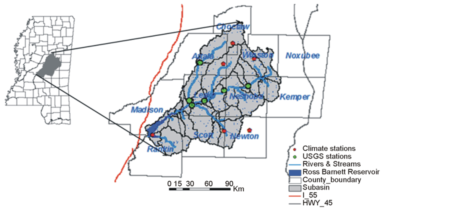
Figure 1. Location map of the Upper Pearl River Watershed showing climate stations, USGS gage stations, highway and reservoir.
The SWAT is a distributed hydrological model, and is characterized with large number of model parameters related to hydrology, water quality, and biomass and crop yields predictions. However, the actual value of many of the model parameters is little known because of the spatial and temporal variability in the processes that are being simulated [13] [14] . As a result, simulated model parameters are often doubted for introducing certain de- gree of uncertainty in the simulated results. Therefore, adjustment of model parameters within their given range is important to obtain close match between simulated and observed values [14] . This can be done by sensitivity analysis (SA) approach which helps to identify and rank parameters that have significant impact on simulated outputs. Thus, it helps in making appropriate selection of parameter(s) during model calibration [15] - [17] .
Sensitivity analysis can be classified as local sensitivity analysis and global sensitivity analysis. Local sensi- tivity analysis, also known as one-at a-time (OAT) approach, involves changing only one parameter at a time by a certain fraction from its base value for identifying model output responses [14] [15] . During this time, other parameters are kept constant and therefore change in the model output during each model simulation is consi- dered as the contribution from parameter that was modified from base [18] [19] . Global sensitivity analysis, in contrast, allows changing random parameters simultaneously over their entire range. A global technique differs from local technique by accounting for variance of the model output associated with model parameter over their entire range of uncertainty [20] . However, if a model is complex and requires large input data, local sensitivity analysis method is preferred over global analysis due to its ease of operation [21] . Many studies in the past have indicated local sensitivity analysis as a good and simple approach for identifying sensitivity of model parameters on the model output [20] [22] [23] . The amount of avilable literature on sensitivity ananlysis of crop paramters for simulation of yield/biomass production using SWAT is still very limited. A study used the SWAT model to conduct sensitivity analysis of crop parameters that influence biomass and yield prediction of switch grass and cotton. Likewise, similar study was conducted to identify sensitive crop parameters for wheat yield calibration [11] . These studies, few in numbers, were primarily focused on identifying parameters sensitive to crop yield prediction of agricultural crops. However, none of these studies have focused on sensitive crop parameters that have significant impact on forest biomass production. The objectives of this study were to conduct: 1) sensitiv- ity analysis of SWAT crop parameters to predict forest biomass production, and 2) performance analysis of SWAT to simulate potential forest biomass production in the Upper Pearl River Watershed.
2. Materials and Methods
2.1. Study Area
This study was conducted in the UPRW, which is located in east-central part of Mississippi (Figure 1) and has an area of approximately 7885 km2. It covers a total of the 11 counties of Mississippi: Choctaw, Attala, Winston, Leake, Neshoba, Kemper, Madison, Rankin, Scott, Newton and Noxubee and flows down to the Ross Barnett Reservoir [8] . The dominant land use of UPRW is forest, which accounts for about 75% of the total watershed area. Longleaf pine, mixed pine-hardwood, dense cypress-Tupelo swamps and bottomland hardwood are the most common types of forest in the watershed [8] . Other land use types of the watershed include pasture (19%), and urban and others (6%). Fine sandy-loam and silt loam are the dominant soil texture of the UPRW. Based on climate data from the National Climatic Data Center during 1980 to 2010, average annual rainfall was about 145 cm with average annual temperature close to 16.3˚C for the watershed. More information about weather stations is described in Section 2.3.
2.2. SWAT Model
The SWAT version 2005 [24] was used for this study. The SWAT is a physically based, watershed scale hydro- logical model that uses various sets of spatial (such as digital elevation model (DEM), landuse, soil) and non-spatial datasets (precipitation, minimum and maximum temperature, wind speed, snow and relative humid- ity) [25] .
The SWAT first delineates and divides the watershed into a number of sub-watersheds, which are further subdivided into hydrologic response units (HRUs). The HRUs are the smallest units in the sub-watershed and are considered to be homogenous with respect to their hydrologic properties [24] [26] . The HRU’s are created by combining unique landuse, soils and topography within sub-watershed [24] .
The SWAT operates on a daily time steps to predict hydrology, water quality and crop growth [27] - [29] . It si- mulates plant biomass and crop yield by using crop growth component, which is a simplified version of Envi- ronmental Policy Integrated Climate (EPIC) model [30] . Accumulation of biomass in SWAT is a function of in- tercepted energy, leaf area index (LAI) and the conversion of intercepted energy into biomass based upon radia- tion use efficiency (RUE). In SWAT, the amount of intercepted daily solar radiation by plant leaf is computed using the Beer’s law (Equation (1)) [24]
 (1)
(1)
where, Hp = intercepted photosynthetically active radiation on a given day, Hday = incident total solar radiation on a given day, k1 = light extinction coefficient, LAI = leaf area index.
The maximum increase in biomass (Δbio) on a given day resulting from the intercepted photosynthetically ac- tive radiation is estimated by using Equation (2) [24] .
 (2)
(2)
where, RUE = radiation use efficiency and is determined from the slope of the regression line between dry mat- ter and cumulative intercepted photosynthetically active radiation [31] . Detail description about SWAT can be found in the SWAT documentation [24] .
2.3. Model Input
The SWAT model requires input of spatial datasets, such as digital elevation model (DEM), soil data, and land use/land cover data. In addition, it also requires non-spatial time series of weather data, such as precipitation, temperature, wind speed, snow and relative humidity. In this study, we used USGS 30 m × 30 m DEM (USGS) [32] for delineating watershed boundary, defining stream network, creating sub-watershed, and for determining topography related information such as slope and angle. The land cover data layer of Year 2009 was obtained from US Department of Agriculture, National Agricultural Statistics Service [33] . The soil database for the study area was created by using State Soil Geographic Database (STATSGO) available within SWAT 2005 da- tabase [34] . The precipitation and temperature data are the weather data used in this study. These data were ob- tained from National Climatic Data Center (NCDC) for a period from 1980 to 2010 [35] . The observed daily precipitation data were obtained from ten rainfall stations: Ackerman, Canton, Carthage, Forest, Gholson, Kos- ciusko, Louisville, Newton, Philadelphia and Walnut Grove. Likewise, observed daily temperature data were obtained from seven climate stations: Carthage, Canton, Forest, Kosciusko, Louisville, Newton and Philadelphia [35] .
2.4. Model Calibration and Validation
The adequacy of SWAT model to accurately simulate forest biomass was first tested by calibrating and validat- ing the model with streamflow data obtained from the six USGS stations: Burnside, Edinburg, Ofahoma, Kos- ciousko, Carthage, and Lena. With an exception of Lena, calibration period at other stations was from 1980- 1995 (16 years) and validation period was from 1996-2008 (13 years). Calibration at Lena station was done from 1998-2002 (5 years) and validation was done from 2003-2008 (6 years). Calibration was done manually by adjusting six streamflow parameters curve number (CN), soil evaporation compensation factor (ESCO), base flow alpha factor (ALPHA_BF), surface runoff lag coefficient (SURLAG), ground water “revap” coefficient (GW_REVAP) and threshold depth of water in the shallow aquifer for baseflow (GWQMIN) (Table 1). During parameter adjustment, different land use types were assigned with different CN value ranging between 70 and 92. The CN value of 77 for deciduous forest, 70 for evergreen forest, 73 for mixed forest, 77 for wetland forest, 79 for pasture, 89 for corn, and 92 for residential medium density showed the maximum model efficiency. In the case of the remaining parameters, same value of respective parameter was assigned for all land use type. For example, the ESCO factor of 0.40, the base flow alpha factor of 0.9, the ground water “revap” coefficient of 0.2, the threshold depth of water in the shallow aquifer of 1000, and the SURLAG coefficient of 1 were assigned for all land use types. These parameters and their values were selected based on the earlier studies conducted in the same watershed [7] and in other similar watersheds [30] [36] [37] . The final value of each model parameter that showed optimal model efficiency during model calibration was used for model validation without their further modification. The streamflow parameters that were selected for model calibration, their range, default value and final value are presented in Table 1.

Table 1. Adjusted parameters’ range, default values, and final values used for streamflow calibration.
2.5. Sensitivity Analysis
Local sensitivity analysis was done for assessing sensitivity of seven crop parameters of SWAT to predict forest biomass production. This was done by changing value of each crop parameter one at a time from its base value, while keeping other parameters constant at their base value. Table 2 shows studied model parameters, their de- finition, base value and their range. The selection of these parameters was based on SWAT manual [24] and ear- lier literatures that have either reported about sensitivity of these parameters for crop yield calibration [11] [38] [39] or have performed sensitivity analysis for crop yield prediction [40] [41] . However, it is important to men- tion that all these past studies were primarily focused on either agricultural crops (cotton, wheat) or bioenergy crops (switchgrass, miscanthus).
The sensitivity of the model to each crop parameter was computed by using relative sensitivity index (Equa- tion (3)) [42] - [46] .
 (3)
(3)
where, Sr is the relative sensitivity index, R is the result or output, P is the model input parameter and b represents the base value. Higher the value of relative sensitivity index, the more sensitive is the SWAT simu- lated biomass to that parameter value. Once the relative sensitivity index of seven crop parameters was obtained, maximum relative sensitivity index of all parameters were compared to determine the most sensitive parameter that affects forest biomass production. Further, all the highest parameters were ranked as highly sensitive, low sensitive, moderately sensitive and no sensitive to forest biomass prediction based on the sensitivity class out- lined by earlier study [28] . The range of sensitivity class used in this study is given in Table 3.
2.6. Forest Biomass Simulation
Forest biomass simulation was performed by adjusting crop parameters within their given range. Provided that the studies related to forest biomass prediction using SWAT is still limited, crop parameters for forest biomass simulation were selected based on the earlier studies related to crop yield prediction for agricultural crops [11] [47] and crop parameters listed in the SWAT manual [24] . According to these studies, BIOE and BLAI are the two important parameters for crop yield prediction, among others. Therefore, during model simulation, these two parameters were modified in the forested HRUs.
The annual average simulated forest biomass of three forest types (deciduous, evergreen and mixed) was compared against the observed forest biomass data obtained from USDA website [46] . The obtained observed data were available at the county level; therefore, to make them consistent with the format of SWAT output,
Table 2. Parameters selected for local sensitivity analysis along with their definition, base value and range.
Table 3. Sensitivity class [28] .
data were adjusted at the sub-basin level by calculating their weighted biomass yield. The biomass data for the UPRW were available for only three different years: 1994, 2006 and 2010. Therefore, based on the range of data available, model was run from 1990-2010 considering first three years as the model warm up period. Simulated forest biomass was then verified against the observed data.
3. Results and Discussion
3.1. Streamflow
The performance of SWAT to predict streamflow was analyzed statistically by using four widely used model ef- ficiency statistics: Coefficient of determination (R2), Nash-Sutcliffe model efficiency index (NSE), root mean square error (RMSE), and percent bias (PBIAS) [7] [47] - [49] . The classification of model performance was done based on the performance rating outlined by earlier studies [49] [50] . The results of model calibration and validation are shown in Table 4. The results indicate fair [47] to very good performance of SWAT for the UPRW, which is indicated by the values of R2 and NSE, ranging from 0.58 to 0.82 and 0.43 to 0.83, respectively (Table 4). Reasonably good performance was also obtained for validation period with values of R2 and NSE ranging from 0.36 to 0.68 and 0.25 to 0.64, respectively (Table 4). These values indicate fair to good correlation between the simulated and observed streamflow during calibration and validation periods.
Furthermore, the values of RMSE that ranged from 13.27 to 39.60 m3/s and 12.31 to 52.44 m3/s during cali- bration and validation period, respectively, also reveal better match between simulated and observed streamflow (Table 4). Even though RMSE is slightly poor at the Carthage and Lena station, other statistics indicate good model performance at these two stations (Table 4). Likewise, values of PBIAS that ranged from −2.70% to −22.91% and −4.89% to −36.98% during calibration and validation periods, respectively, also illustrate good fit between simulated and observed streamflow. These values, however, suggest that the model has overestimated bias at all the six stations during calibration period and at the three stations (Kosciousko, Lena and Ofahoma) during validation period, respectively. Possible explanations for such discrepancies between different stations for streamflow prediction may be due to the variation of precipitation input at these stations.
The model efficiency statistics computed in this study for the monthly streamflow prediction are found to be in general agreement with those reported by earlier studies using the SWAT model [7] [29] [36] [50] - [52] . A study conducted in southeast Indiana reported calibrated monthly streamflow NSE values between 0.59 and 0.80 for three different watersheds [52] . Likewise, a study determined R2 = 0.81, NSE = 0.56, and PBIAS = −95.06% for calibrated monthly streamflow for Red Rock Creek watershed in south-central Kansas [50] . Moreover,
Table 4. Model performance during streamflow calibration and validation.
SWAT model performance in this study is also consistent with the performance statistics reported by a study conducted in the same watershed [7] . The values of R2, NSE and RMSE estimated at the five USGS gauge sta- tions were reported between 0.69 m3/s and 0.79 m3/s, 0.68 m3/s and 0.79 m3/s, and 14.14 m3/s and 37.03 m3/s, respectively. Thus because of the good performance shown by the model in this study, the calibration SWAT model was further used to perform sensitivity analysis of crop parameters as well as to evaluate SWAT’s per- formance to predict potential forest biomass production in the UPRW.
Figure 2 illustrates the relative sensitivity of studies crop parameters. The Y-axis represents the relative sen- sitivity index and the X-axis represents parameter values that were varied over their entire range. Visual analysis of Figure 2 indicates that DLAI, BIOE, BLAI and RDMX showed positive relative sensitivity and FRGRW1, LAIMX1 and CHTMX showed negative relative sensitivity. Furthermore, it also indicates that relative sensitivi- ty of parameters such as DLAI, BIOE, BLAI, RDMX, CHTMX increases with decrease in value from their base value. On the contrary, relative sensitivity of parameter FRGRW1 seems to be increasing when its value was in- creased from 0.25 to 0.45. However, further increase in its value causes decrease in the relative sensitivity. Si- milarly, relative sensitivity of LAIMX1 increases with increase its value from 0.25 to 0.65, but further increase in value from its base value decreases the relative sensitivity.
3.2. Model Sensitivity to Crop Parameters
Figure 3 demonstrates all the highest relative sensitivity index of each crop parameter. Results indicate that the relative sensitivity of studied parameters varied between no sensitivity (Sr = −0.0080) to moderately sensitivity (Sr = 0.44). Figure 3 shows that only three parameters: DLAI, BIOE and BLAI are sensitive (with relative sen- sitivity greater than 0.1). Further classification of relative sensitivity index using sensitivity class outlined by earlier study [28] , DLAI and BIOE were only moderately sensitive and BLAI shows low sensitivity with relative sensitivity index of 0.44, 0.35 and 0.14, respectively (Table 2). Other parameters: RDMX, FRGRW1, CHTMX and LAIMX1, though they directly impact the amount of light intercepted by leaves, were not found to be sensi- tive in predicting forest biomass production.
Our results on the value of relative sensitivity for all studied parameters appear to be lower than the values reported by past study for switch grass and miscanthus [41] . In contrast to our finding, BIOE and BLAI were reported as the most sensitive parameter followed by the DLAI [41] . On the other hand, with an exception of BLAI, our finding appears to be consistent with earlier study [41] if the relative sensitivity shown by each para- meter is classified in accordance with sensitivity class outlined by another study [28] . It is worth mentioning that due to the limited availability of studies related to sensitivity analysis of SWAT crop parameter for forest bio- mass prediction, comprehensive comparison of relative sensitivity showed by each studied parameters for forest biomass production is limited in this study.
3.3. Forest Biomass Production Potential
Forest biomass simulated with the default value of selected crop parameters resulted in poor model performance due to their much lower prediction. Therefore, increasing the value of simulated forest biomass was the main focus of this study during forest biomass simulation. For this purpose, selected parameters were modified gradu- ally from their base following the sequence of sensitivity shown by these parameters during sensitivity analysis.
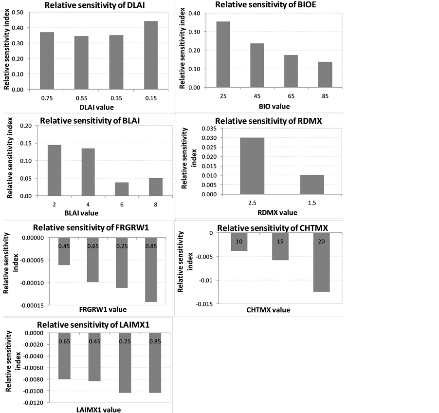
Figure 2. Relative sensitivity of selected crop parameters within their tested range.
It was observed that increasing the value of BIOE and BLAI resulted in increase forest biomass, whereas in- creasing the value of DLAI shows opposite result. Forest biomass remained unchanged when other parameters were modified, which was expected, because these parameters were not sensitive at the time of sensitivity analy- sis. Hence, these parameters including DLAI were set to their default value at the time of final simulation process.
The BIOE value in this study was increased gradually and was finally set to 75. On the contrary, other studies related with yield prediction of agricultural crops were found to have reduced the value of BIOE because, in their study, the default value resulted in higher yield [45] [53] . Additionally, the value of BLAI was also gradu- ally increased and was set to 8 as it resulted in good agreement between observed and simulated data. The final value of BLAI for forested area was selected following the earlier literature [54] .
The results demonstrate good correlation (R2 = 0.83) between simulated and observed biomass. Visual analy- sis of Figure 4 demonstrates that except in Year 1994, simulated forest biomass is lower than observed biomass. Similarly, minimum degree of average error (RMSE = 11.11 Mg/ha) between simulated and observed forest biomass data. The finding of this study also shows that the UPRW has the potential to produce approximately 49 Mg/ha of average forest biomass annually (Figure 4). This value is less by 3 Mg/ha (approximately 6%) than the average observed forest biomass in the study area. It is important to note that 85% of total available biomass can be sustainably obtained for bioenergy using an integrated system [55] .
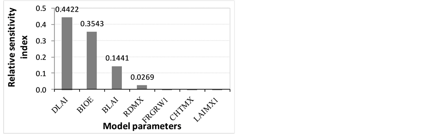
Figure 3. Overall relative sensitivity index of studied crop parameters.
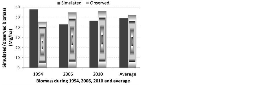
Figure 4. Comparison of observed versus simulated forest biomass during 1994, 2006, 2010 and average.
Following this logic, approximately 42 Mg/ha of forest biomass can be sustainably recovered for bioenergy production from the UPRW. However, given the incipient bioenergy market and conventional use of biomass in forest product industries, actual biomass available for bioenergy use cannot be predicted as such.
4. Conclusions
Results on SWAT performance to predict streamflow revealed satisfactory performance (R2 and NSE > 0.6) and low value of PBIAS and RMSE. Furthermore, results on local sensitivity analysis of seven crop parameters to predict forest biomass production determine three parameters: DLAI, BIOE and BLAI as sensitive to predict forest biomass production. DLAI and BIOE are moderately sensitive and BLAI shows low sensitivity. In con- trast to the sensitivity analysis conducted in switchgrass and miscanthus, relative sensitivity of all studied para- meters in this study has shown lower value of relative sensitivity index. Thus, sensitivity analysis conducted in this study provides baseline information about the sensitivity of seven crop parameters of SWAT to influence forest biomass production and, therefore, may serve as a basis for similar future research.
Likewise, SWAT adequately predicted potential forest biomass for the UPRW with high value of R2 (0.83), small difference (<6%) between predicted and observed mean and low RMSE value (11.11 Mg/ha). Results fur- ther indicate that the UPRW has the potential to produce approximately 49 Mg/ha of average annual forest bio- mass, which is slightly less (3 Mg/ha or 6%) than the average observed forest biomass in the study area. Overall, this study demonstrated that SWAT can be a useful tool for modeling the availability of forest biomass as a po- tential bioenergy feedstock. However, further studies using additional data were recommended to better analyze the performance of SWAT in simulating the availability of potential forest biomass.
Acknowledgements
This material is based upon the work performed through the special Research Initiatives (SRI) at Mississippi Agricultural and Forestry Experiment Station (MAFES); the Sustainable Energy Research Centre at Mississippi State University; and is supported by the Department of Energy under Award number DE-FG3606GO86025. We acknowledge the contributions Mr. Kurt Readus, Assistant State Conservationist, NRCS/MS.
References
- Bartuska, A. (2006) Why Biomass Is Important―The Role of the USDA Forest Service in Managing and Using Bio- mass for Energy and Other Uses. http://www.fs.fed.us/research/pdf/biomass_importance.pdf.
- Joshi, O. and Mehmood, S.R. (2011) Factors Affecting Nonindustrial Private Forest Landowners’ Willingness to Sup- ply Woody Biomass for Bioenergy. Biomass and Bioenergy, 35, 186-192. http://dx.doi.org/10.1016/j.biombioe.2010.08.016
- Sissine, F. (2007) Energy Independence and Security Act of 2007: A Summary of Major Provisions. CRS Report for Congress. http://www.seco.noaa.gov/Energy/2007_Dec_21_Summary_Security_Act_2007.pdf
- Parresol, B.R. (1999) Assessing Tree and Stand Biomass: A Review with Examples and Critical Comparisons. Forest Science, 45, 573-593.
- Lu, D. (2006) The Potential and Challenge of Remote Sensing Based-Biomass Estimation. International Journal of Remote Sensing, 27, 1297-1328. http://dx.doi.org/10.1080/01431160500486732
- Main-Knorn, M., Moisen, G.G., Healey, S.P., Keeton, W.S., Freeman, E.A. and Hostert, P. (2011) Evaluating the Re- mote Sensing and Inventory-Based Estimation of Biomass in the Western Carpathians. Remote Sensing, 3, 1427-1446. http://dx.doi.org/10.3390/rs3071427
- Parajuli, P.B. (2010) Assessing Sensitivity of Hydrologic Responses to Climate Change from Forested Watershed in Mississippi. Hydrological Processes, 24, 3785-3797.
- Mississippi Department of Environmental Quality (MDEQ) (2007) Citizen’s Guide to Water Quality in the Pearl River Basin. http://www.deq.state.ms.us/mdeq.nsf/0/9EC5A103F2D7D183862574FD005382FA/$file/Pearl+River+Basin_Final_pr.pdf?OpenElement
- Wang, X., Harmel, R.D., Williams, J.R. and Harman, W.L. (2005) Evaluation of EPIC for Assessing Crop Yield, Ru- noff, Sediment and Nutrient Losses from Watersheds with Poultry Litter Fertilization. Transactions of the ASABE, 49, 47-49. http://dx.doi.org/10.13031/2013.20243
- Baskaran, L., Jager, H.I., Schweizer, P.E. and Srinivasan, R. (2010) Progress toward Evaluating the Sustainability of Switchgrass as a Bioenergy Crop Using the SWAT Model. Transactions of the ASABE, 53, 1547-1556. http://dx.doi.org/10.13031/2013.34905
- Faramarzi, M., Yanga, H., Schulinc, R. and Abbaspoura, K.C. (2010) Modeling Wheat Yield and Crop Water Produc- tivity in Iran: Implications of Agricultural Water Management for Wheat Production. Agricultural Water Management, 97, 1861-1875. http://dx.doi.org/10.1016/j.agwat.2010.07.002
- Srinivasan, R., Zhang, X. and Arnold, J. (2010) SWAT Ungauaged: Hydrological Budget and Crop Yield Predictions in the Upper Mississippi River Basin. Transactions of the ASABE, 53, 1533-1546. http://dx.doi.org/10.13031/2013.34903
- Cibin, R., Sudheer, K.P. and Chaubey, I. (2010) Sensitivity and Identifiability of Stream Flow Generation Parameters of the SWAT Model. Hydrological Processes, 24, 1133-1148. http://dx.doi.org/10.1002/hyp.7568
- Holvoet, K., van Griensven, A., Seuntjens, P. and Vanrolleghem, P.A. (2005) Sensitivity Analysis for Hydrology and Pesticide Supply towards the River in SWAT. Physics and Chemistry of the Earth, 30, 518-526. http://dx.doi.org/10.1016/j.pce.2005.07.006
- Saltelli, A., Tarantola, S., Campolongo, F. and Ratto, M. (2004) Sensitivity Analysis in Practice: A Guide to Assessing Scientific Models. John Wiley and Sons Ltd., Hoboken.
- Kalin, L. and Hantush, M.M. (2006) Hydrologic Modeling of an Eastern Pennsylvania Watershed with NEXRAD and Rain Gauge Data. Journal of Hydrologic Engineering, 11, 555-569. http://dx.doi.org/10.1061/(ASCE)1084-0699(2006)11:6(555)
- Haan, C.T. and Skaggs, R.W. (2003) Effect of Parameter Uncertainty on DRAINMOD Predictions: I. Hydrology and Yield. Transactions of the ASAE, 46, 1061-1067.
- van Griensven, A. and Meixner, T. (2006) Methods to Quantify and Identify the Sources of Uncertainty for River Ba- sin Water Quality Models. Water Science Technology, 53, 51-59
- Soutter, M. and Musy, A. (1999) Global Sensitivity Analyses of Three Pesticide Leaching Models Using a Monte-Car- lo Approach. Journal of Environmental Quality, 28, 1290-1297. http://dx.doi.org/10.2134/jeq1999.00472425002800040033x
- Pathak, T.B., Fraisse, C.W., Jones, J.W., Messina, C.D. and Hoogenboom, G. (2007) Use of Global Sensitivity Analy- sis for CROPGRO Cotton Model Development. Transactions of the ASABE, 50, 2295-2302. http://dx.doi.org/10.13031/2013.24082
- Patric, J.H., Evans, J. and Helvey, J.D. (1984) Summary of Sediment Yield Data from Forested Land in the United States. Journal of Forestry, 82, 101-104.
- Graff, C.D., Sadeghi, A.M., Lowrance, R.R. and Williams, J.R. (2005) Quantifying the Sensitivity of the Riparian Eco- system Management Model (REMM) to Changes in Climate and Buffer Characteristics Common to Conservation Practices. Transactions of the ASAE, 48, 1377-1387. http://dx.doi.org/10.13031/2013.19195
- Sarkar, S., Miller, S.A., Frederick, J.R. and Chamberlain, J.F. (2011) Modeling Nitrogen Loss from Switchgrass Agri- cultural systems. Biomass and Bioenergy, 35, 4381-4389. http://dx.doi.org/10.1016/j.biombioe.2011.08.009
- Neitsch, S.L., Arnold, J.G., Kiniry, J.R. and Williams, J.R. (2005) Soil and Water Assessment Tool SWAT, Theoreti- cal Documentation. Blackland Research Center, Grass-Land, Soil and Water Research Laboratory, Agricultural Re- search Service, Temple.
- Arnold, J.G., Srinivasan, R., Muttiah, R.S. and Williams, J.R. (1998) Large Area Hydrologic Modeling and Assess- ment Part I: Model Development. JAWRA: Journal of American Water Resources Association, 34, 73-89. http://dx.doi.org/10.1111/j.1752-1688.1998.tb05961.x
- Eckhardt, K. and Arnold, J.G. (2001) Automatic Calibration of a Distributed Catchment Model. Journal of Hydrology, 251, 103-109. http://dx.doi.org/10.1016/S0022-1694(01)00429-2
- Borah, A.K. and Bera, M. (2003) Watershed-Scale Hydrological and Nonpoint-Source Pollution Models: Review of Mathematical Bases. Transactions of the ASAE, 46, 1553-1566. http://dx.doi.org/10.13031/2013.15644
- Lenhart, T., Eckhardt, K., Fohrer, N. and Frede, H.G. (2002) Comparison of Two Different Approaches of Sensitivity Analysis. Physics and Chemistry of the Earth, Parts A/B/C, 27, 645-654. http://dx.doi.org/10.1016/S1474-7065(02)00049-9
- Spruill, C.A., Workman, S.R. and Taraba, J.L. (2000) Simulation of Daily and Monthly Stream Discharge from Small Watersheds Using the SWAT Model. Transactions of the ASAE, 43, 1431-1439. http://dx.doi.org/10.13031/2013.3041
- Gassman, P.W., Reyes, M.R., Green, C.H. and Arnold, J.G. (2007) The Soil and Water Assessment Tool: Historical Development, Applications and Future Research Directions. Transactions of the ASABE, 50, 1211-1250. http://dx.doi.org/10.13031/2013.23637
- Kiniry, J.R., Tischler, C.R. and Van Esbroeck, G.A. (1999) Radiation Use Efficiency and Leaf CO2 Exchange for Di- verse C4 Grasses. Biomass and Bioenergy, 17, 95-112. http://dx.doi.org/10.1016/S0961-9534(99)00036-7
- US Geological Society (USGS) (1999) National Elevation Data-Set. http://seamless.usgs.gov/website/seamless/viewer.htm
- US Department of Agriculture, National Agricultural Statistics Service (USDA/NASS) (2009) The Cropland Data Layer. http://www.nass.usda.gov/research/Cropland/SARS1a.htm
- US Department of Agriculture (USDA) (2005) Soil Data Mart. Natural Resources Conservation Service. http://datagateway.nrcs.usda.gov/
- National Climatic Data Center (NCDC) (2010) Locate Weather Observation Station Record. http://www.ncdc.noaa.gov/land-based-station-data/find-station
- Saleh, A., Williams, J.R., Wood, J.C., Hauck, L.M. and Blackburn, W.H. (2004) Application of APEX for Forestry. Transactions of the ASAE, 47, 751-765. http://dx.doi.org/10.13031/2013.16107
- Santhi, C., Arnold, J.G., Williams, J.R., Dugas, W.A. and Hauck, L. (2001) Validation of the SWAT Model on a Large Rwer Basin with Point and Nonpoint Sources. JAWRA: Journal of American Water Resources Association, 37, 1169- 1188. http://dx.doi.org/10.1111/j.1752-1688.2001.tb03630.x
- Breuer, L., Eckhardt, K. and Frede, H.G. (2003) Plant Parameter Values for Models in Temperate Climates. Ecological Modeling, 169, 237-293. http://dx.doi.org/10.1016/S0304-3800(03)00274-6
- Eckhardt, K., Breuer, L. and Frede, H.G. (2003) Parameter Uncertainty and the Significance of Simulated Land Use Change Effects. Journal of Hydrology, 273, 164-176. http://dx.doi.org/10.1016/S0022-1694(02)00395-5
- Akhavana, S., Abedi-Koupaia, J., Mousavia, S.F., Afyunib, M., Eslamiana, S.S. and Abbaspour, K.C. (2010) Applica- tion of SWAT Model to Investigate Nitrate Leaching in Hamadan Bahar Watershed, Iran. Agriculture, Ecosystem and Environment, 139, 675-688. http://dx.doi.org/10.1016/j.agee.2010.10.015
- Chaubey, I., Raj, C., Trybula, E., Frakenberger, J., Brouder, S. and Volencec, J. (2011) Improving the Simulation of Biofuel Crop Sustainability Assessment Using SWAT Model. http://swat.tamu.edu/media/39263/chaubey.pdf
- James, L.D. and Burges, S.J. (1982) Selection, Calibration, and Testing of Hydrologic Models. In: Haan, C.T., Johnson, H.P. and Brakensiek, D.L., Eds., Hydrologic Modeling of Small Watersheds, ASAE Monograph, St. Joseph, 437-472.
- Jesiek, J.B. and Wolf, D.D. (2005) Sensitivity Analysis of the Virginia Phosphorus Index Management Tool. Transac- tions of the ASAE, 48, 1773-1781. http://dx.doi.org/10.13031/2013.20011
- White, K.L. and Chaubey, I. (2005) Sensitivity Analysis, Calibration and Validation for a Multisite and Multivariable SWAT Model. JAWRA: Journal of American Water Resources Association, 41, 1077-1089. http://dx.doi.org/10.1111/j.1752-1688.2005.tb03786.x
- Nair, S.S., King, K.W., Witter, J.D., Sohngen, B.L. and Fausey, N.R. (2011) Importance of Crop Yield in Calibrating Watershed Water Quality Simulation Tools. JAWRA: Journal of American Water Resources Association, 47, 1285- 1297. http://dx.doi.org/10.1111/j.1752-1688.2011.00570.x
- USDA Forest Service (2011) Forest Inventory Data Online (FIDO). http://www.fia.fs.fed.us/tools-data/
- Nash, J.E. and Sutcliffe, J.V. (1970) River Flow Forecasting through Conceptual Models: Part I. A Discussion of Prin- ciples. Journal of Hydrology, 10, 282-290. http://dx.doi.org/10.1016/0022-1694(70)90255-6
- Gupta, H.V., Sorooshian, S. and Yapo, P.O. (1999) Status of Automatic Calibration for Hydrologic Models: Compari- son with Multilevel Expert Calibration. Journal of Hydrologic Engineering, 4, 135-143. http://dx.doi.org/10.1061/(ASCE)1084-0699(1999)4:2(135)
- Moriasi, D.N., Arnold, J.G., Van Liew, M.W., Binger, R.L., Harmel, R.D. and Veith, T.L. (2007) Model Evaluation Guidelines for Systematic Quantification of Accuracy in Watershed Simulations. Transactions of the ASABE, 50, 885- 900. http://dx.doi.org/10.13031/2013.23153
- Parajuli, P.B., Nelson, N.O., Frees, L.D. and Man-Kin, K.R. (2009) Comparison of AnnAGNPS and SWAT Model Si- mulation Results in USDACEAP Agricultural Watersheds in South-Central Kansas. Hydrological Processes, 23, 748- 763.
- Nejadhashemi, A.P., Wardynski, B.J. and Munoz, J.D. (2011) Evaluating the Impacts of Land Use Changes on Hydro- logic Responses in the Agricultural Regions of Michigan and Wisconsin. Hydrology and Earth System Sciences Discu- ssions, 8, 3421-3468. http://dx.doi.org/10.5194/hessd-8-3421-2011
- Vazquez-Amábile, G.G. and Engel, B.A. (2005) Use of SWAT to Compute Groundwater Table Depth and Streamflow in the Muscatatuck River Watershed. Transactions of the ASAE, 48, 991-1003. http://dx.doi.org/10.13031/2013.18511
- Baumgart, P. (2005) Loads to Green Bay from the Lower Fox River Subbasin Using the Soil and Water Assessment Tool (SWAT). http://www.uwgb.edu/watershed/reports/related_reports/load-allocation/lowerfox_tss-p_load-allocation.pdf
- Fohrer, N., Möller, D. and Steiner, N. (2002) An Interdisciplinary Modeling Approach to Evaluate the Effects of Land Use Change. Physics and Chemistry of the Earth, Parts A/B/C, 27, 655-662. http://dx.doi.org/10.1016/S1474-7065(02)00050-5
- Perlack, R.D., Wright, L.L. Turhollow, A.F. Graham, R.L., Stokes, B.J. and Erbach, D.C. (2005) Biomass as Feedstock for a Bioenergy and Bioproducts Industry: The Technical Feasibility of a Billion-Ton Annual Supply. Department of Energy, Oak Ridge. http://dx.doi.org/10.2172/885984
NOTES

*Corresponding author.