Modeling and Numerical Simulation of Material Science
Vol.4 No.3(2014), Article
ID:47695,15
pages
DOI:10.4236/mnsms.2014.43012
Micromechanical Analysis of Thermal Expansion Coefficients
Christian Karch
Airbus Group Innovations, Munich, Germany
Email: christian.karch@eads.net
Copyright © 2014 by author and Scientific Research Publishing Inc.
This work is licensed under the Creative Commons Attribution International License (CC BY).
http://creativecommons.org/licenses/by/4.0/


Received 4 May 2014; revised 3 June 2014; accepted 2 July 2014
ABSTRACT
Thermal expansion coefficients play an important role in the design and analysis of composite structures. A detailed analysis of thermo-mechanical distortion can be performed on microscopic level of a structure. However, for a design and analysis of large structures, the knowledge of effective material properties is essential. Thus, either a theoretical prediction or a numerical estimation of the effective properties is indispensable. In some simple cases, exact analytical solutions for the effective properties can be derived. Moreover, bounds on the effective values exist. However, in dealing with complex heterogeneous composites, numerical methods are becoming increasingly important and more widely used, because of the limiting applicability of the existing (semi-)analytical approaches. In this study, finite-element methods for the calculation of effective thermal expansion coefficients of composites with arbitrary geometrical inclusion configurations are discussed and applied to a heterogeneous lightning protection coating made from Dexmet® copper foil 3CU7-100FA and HexPly® epoxy resin M21. A short overview of some often used (semi-)- analytical formulas for effective thermal expansion coefficients of heterogeneous composites is given in addition.
Keywords:Micromechanics, Thermal Expansion, Representative Volume Element, Finite-Element Method

1. Introduction
In continuum mechanics, the materials are considered as ideal, continuous, and homogenous media. Within the framework of continuum mechanics, the response of homogenous material to an external load is described by appropriate constitutive relations without recourse to any microstructural considerations. In fact, all materials are inhomogeneous on sufficient small, microscopic scale. The continuum is only a model of materials in the macroscopic scale. Therefore, the homogeneity of materials depends on the scale of examination.
Heterogeneous materials exist in both synthetic products and nature. An important class of synthetic heterogeneous materials is the class of composites manufactured as mixture of two or more constituents. The heterogeneous composites can have anisotropic properties for different domains and/or directions due to the difference of the material properties of their constituents. This is an important feature of heterogeneous composites which is generally used to design new materials to meet various desired properties and functions which are absent in their constituents. Composite heterogeneous materials often exhibit complex properties presenting new challenges and opportunities not only for excellent mechanical but also for thermal, electric, and chemical applications.
The present study focuses on determining the effective linear thermal expansion coefficient (CTE) of heterogeneous composite materials. In modern technique, it is necessary to consider the influence of temperature on toughness and stability of structures. The thermal expansion behaviour is particularly important when composite materials are used in conjunction with other materials and when it is necessary to match the CTE of one structural component with another. The effective property is actually the property of a hypothetical homogeneous material which yields the same global response as that of the complex heterogeneous one at the same given conditions and loads. Ideally, the averaging process for deriving the effective properties takes into account the properties of all constituents of the complex heterogeneous system and their interactions. The actual averaging process to obtain effective properties has to be specified carefully. In some simple cases, it is possible to obtain exact analytical solutions for the effective properties. When this is not feasible, it is at least possible to obtain analytical bounds on the effective values. Because of the limiting applicability of the existing analytical approaches the numerical methods are becoming increasingly important and more widely used. The FEM has become very popular, especially when the exact (known) geometry of the constituents (and the thermo-mechanical history-preloads-of the composite) can be incorporated into the simulation of the effective properties. One common approach is to use a unit-cell model (RVE), where one or more types of reinforcements, fibres or particles, are embedded within a matrix material, to simulate a complex heterogeneous composite with a periodic array constituents. In such a way, it is possible to simulate the true microstructures taking into account the topology, morphology and clustering of reinforcement constituents.
2. Averaging and Homogenization
In continuum mechanics, the materials are considered as ideal, continuous, and homogenous media. Within the framework Homogenization from intuitive viewpoint is described in the review article of Hashin [1] and in the book of Nemat-Nasser [2] . Three length scales are introduced (see Figure 1):
Ÿ The microscale is characterized by lengths less than l3, which is generally chosen greater than the maximum size of the inhomogeneity in the microstructure.
Ÿ The intermediate mesoscopic length scale is characterized by length l2, at which the composite material appears statistically homogeneous, and at which the macroscopic fields have a slow variation.
Ÿ The macroscale is characterized by lengths greater then l1, which is less than the relevant dimension of the considered body and less than the scale of variations in the macroscopic structure of the composite.
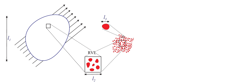
Figure 1. Homogenization procedure of a heterogeneous composite.
Most micromechanical models are explicitly based on the assumption that the length scales in a given composites differ substantially: . That means that, on the one hand, the fluctuating contributions to the considered fields (stress, strain, etc.) at the smaller length scale (fast variables) influence the behaviour at the larger length scale only via their volume averages. On the other hand, gradients of the fields as well as compositional gradients at the larger length scale (slow variables) are not significant at the smaller length scale, where these fields appear to be locally constant and can be described in terms of uniform applied fields. Formally, this splitting of the fields into slow and fast contributions can be written as
 , (1)
, (1)
where
 is the macroscopic slowly varying field, whereas
 stands for the microscopic fluctuations. The smoothing operation of local averaging on the mesoscale is given by
 , (2)
, (2)
where V defines a mesosized volume element of the heterogeneous composite considered. The homogenization volume should be chosen to be a proper RVE of sufficient size on the mesoscale to contain all information necessary for describing the microscopic behaviour of the heterogeneous composite. RVE elements are sometimes defined by requiring them to be statistically representative of the microgeometry of the composites. Such geometrical RVEs are independent of the physical property of the composite to be studied. Sometimes the choice of the RVE is based on the requirement that the overall responses with respect to applied external excitations are independent of the actual position and orientation of the RVE (see Hill [3] ). Thus, the RVE must be sufficiently large to allow a meaningful sampling of the microscopic fields and sufficiently small for the influence of macroscopic gradients to be negligible. However, the size of the RVE is restricted by the computational effort needed for the determination of the microscopic fields. It has been verified that the periodic boundary conditions provide a better estimation of the overall properties, than the uniform displacement or uniform traction boundary conditions (see e.g. Geers [4] ). Increasing the size of the microstructural cell leads to a better estimation of the effective properties, and, finally, to a convergence of the results obtained with the different boundary conditions, as schematically shown in Figure 2.
3. Coefficients of Thermal Expansion
Most natural materials, with very few exceptions in narrow temperature range, expand when heated. This is caused by the atomic or molecular vibrations at all temperatures. The amplitude and the population of density of states of these vibrations (phonons) increase with increasing temperature. The linear coefficient of thermal expansion α is defined as
 , (3)
, (3)
where the strain e and the linear CTE a are second-rank symmetric tensors. Over a small temperature range of DT the strain e can be assumed directly proportional to the linear coefficient of the thermal expansion a and the
 (a)
(a)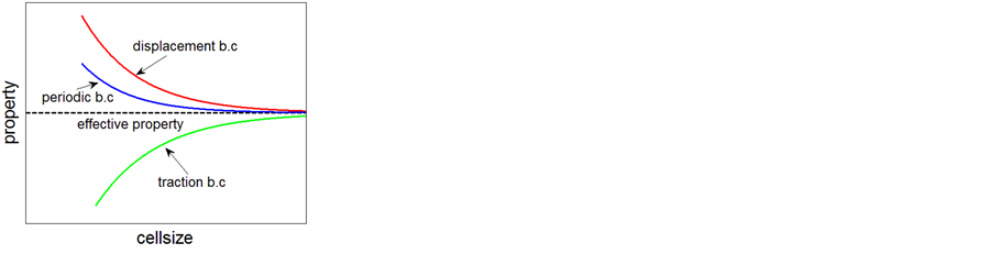 (b)
(b)
Figure 2. (a) Several RVEs of different sizes of a random composite; (b) Schematic convergence.
constitutive relationship between stress s and strain e and temperature change DT is given by the DuhamelNeumann law
 . (4)
. (4)
The constitutive equation contains the components of the fourth-order stiffness tensor Cijkl1. In the following the investigation is restricted to materials with at least orthotropic symmetry. With the contracted Voigt notation the Duhamel-Neumann law can be written in matrix form with the stiffness C as a 6 ´ 6 symmetric second-order (matrix) tensor and the stress {s} and strain fields {e} as column vectors, see e.g. Hyer [5] .
4. Analytical and Semi-Analytical Approaches
The development of homogenization techniques for the purpose of predicting the effective material properties of heterogeneous composite materials is an on-going process. Many analytical and semi-empirical formulas have been derived to evaluate the effective coefficient of the linear thermal expansion of different types of heterogeneous composites. Some formulas are briefly mentioned in following sections. Most of available formulas are restricted to heterogeneous composites made from isotropic phases.
4.1. Mixture Rules: Voigt and Reuss Bounds
The rule-of-mixture models are derived from the assumption of uniform strain or stress of the composite structure. The Voigt [6] upper bound for the effective thermal expansion coefficient α* is given by
 , (5)
, (5)
where xi, Ei, and αi are the volume fractions, the elastic moduli, and the coefficients of thermal expansions of the single isotropic phases of the composites, respectively.
Reuss [7] assumption of uniform stress in the composite materials simply gives
 . (6)
. (6)
For unidirectional fibre reinforced composite Equation (5) gives a reasonable approximation for the effective thermal expansion coefficient in fibre direction (E1 and α1 are then replaced by the longitudinal modulus E1L and the longitudinal thermal expansion α1L of the fibre, respectively). Equation (6) may be used as an upper bound for prediction of the effective transverse thermal expansion coefficient (α1 is then replaced simple by the transverse thermal expansion coefficient of the fibre α1T). However, this is generally a poor approximation for the effective transverse thermal expansion coefficient.
4.2. Turner Approach
Turner model [8] takes into account the mechanical interaction between the phases in the heterogeneous composite material. The expression given by Turner is somehow similar to that derived by Voigt. However, the Young modulus E is replaced by the bulk modulus K
 . (7)
. (7)
Moreover, the Turner formula is used as a lower bound for the effective CTE and not as the upper bound like the Voigt formula.
4.3. Levin Formula
Levin model [9] gives an effective CTE for a composite made from isotropic constituents
 . (8)
. (8)
However, in order to determine the value of the CTE the effective value of the bulk modulus of the heterogeneous composite K* has to be known. The Levin formula is often used to determine the upper and lower bounds of the CTE by using an effective elastic models that give bounds for K* (see e.g. Hashin-Shtrikman [10] ). The extension of Levin formula for two-phase composites made from anisotropic phases is given in Appendix.
4.4. Rosen and Hashin Formula
The Levin formula was extended to anisotropic heterogeneous composites made from anisotropic constituents by Rosen and Hashin [11]
 , (9)
, (9)
where
 . (10)
For isotropic constituents the above equation can be simplified to
 . (11)
The heterogeneous composite, made from the isotropic constituents, needs not to be isotropic.
4.5. Schapery Model
Schapery [12] used elastic energy principles to derive bounds for effective CTEs of anisotropic composites made from isotropic constituents. The lower and upper bounds for the effective coefficients are given by
 , (12)
where j takes the values 1, 2, and 3.
 is the value of the effective uniaxial elasticity modulus
 and
and
 represents the largest possible error if the mean value between upper and lower bounds is used (
 set to 0)
 . (13)
The EU and EL are upper and lower bounds of the effective elasticity uniaxial moduli
 . (14)
Schapery [12] showed that the above results lead to simple, approximate formulas for unidirectional, fibre-reinforced composites. For composite made from isotropic phases the transverse thermal expansion coefficients is approximately given by
 . (15)
This equation is very often cited as Schapery equations for transverse CTE. However, it is taken from the publication Van Fo Fly [13] and adapted to the particular case of fibre-reinforced transverse isotropic composites.
4.6. Budiansky Self-Consistent Formula
Budiansky formula for random mixtures of N isotropic phases is based on self-consistent equivalent medium approach [14]
 , (16)
with
 . (17)
The above equations are used to determine the effective thermal expansion coefficient
 . (18)
In order to determine the value of the CTE the effective values of the bulk K* and the shear modulus G* of the heterogeneous composite have to be determined too.
4.7. Chamberlain’s Model
A model for the transverse thermal expansion of unidirectional transverse-isotropic composites was derived by Chamberlain [15] . The equation for the longitudinal thermal expansion coefficient is identical to Voigt [6] upper bounds, see Equation (5). The expression for the CTE in the transverse direction takes the form
 , (19)
where “1” refers to matrix and “2” refers to fibres. F is the geometrical packing factor and is equal to 0.9069 (0.7854) for hexagonal (square) fibres arrays
5. Finite Element Modelling
Finite element methods (FEM) are applied to solve numerically differential equations that are difficult or impossible to solve analytically. The FEM takes a given geometry and breaks it down into smaller parts (elements) and uses a system of algebraic equation to describe the relationships at the nodes connecting the neighbouring elements. This procedure allows transforming the original differential equations into a system of algebraic equations that can be numerically solved to come up with an approximate numerical solution to the original problem.
The validity of the homogeneity assumption depends on the detailed microstructure at scale of the individual phases and thus the proper selection of the RVE. The local value of the volume fraction of constituents varies with the size and location of the sample region over which the volume fractions are computed. The values of volume fractions can scatter when the sample volume is too small; the scattering factor decreases as the sample volume increases. In the theory of homogenization (of random heterogeneous composites), the volume fractions are the key parameters on which other properties are based. Thus, in principle, the minimum sample volume over which the volume fractions are independent of the sample location should be considered as the minimal RVE. When the heterogeneous composite specimen is subjected for example to a uniform mechanical loading, each RVE will undergo identical deformation-a certain periodicity then exists in the displacement, stress and strain fields. In order to determine the effective properties the induced microscopic fields within the RVE need to be determined (semi-)analytically or numerically.
The RVE approach assumes that the analysed microstructure is periodic in one, two, or three dimensions. In this case, a single periodic RVE represents the composite material considered. The boundary conditions, however, must assure the periodic deformation of the boundaries regardless of the applied load. Hence, for FEM simulation the term periodic BC means actually a periodic coupling of degrees of freedom on corresponding nodes of the opposite boundaries in addition to other loads or displacements. An example of a typical 2D RVE is depicted in Figure 3.
For the 2D RVE shown in the figure above, the periodicity condition may be recast into the following constraint relations
 . (20)
where xL, xR, xB and xT denote a position vector on the left, right, bottom and top boundary of the RVE, respectively; xi, i = 1, 2, 3, 4 are the position vectors of the corner nodes in the deformed state. That means that the nodes 1, 2 and 1, 4 (and so on) are coupled by constraint equations. Moreover, it is possible to couple the displacements of the boundary nodes to master nodes (di)
 . (21)
This is a smart way to tie the displacements of all boundary nodes to master nodes and to gain the reaction of the RVE to the applied loads form the reaction of these master nodes. For a determination of the CTEs a uniform temperature load is applied on the entire 3D RVE. The coefficients of thermal expansion are finally determined using equation below
 , (22)
where the displacements for the calculation of the strains are obtained from the FE solution for the master nodes. The advantage of this approach (AP1) is that it generally applicable even for non-symmetric RVEs. The reactions (i.e., strains) of the RVEs to the applied loads can simply be extracted from the reactions (i.e., strains) of the master nodes. However, this approach has some disadvantages: the complete RVE has to be meshed for the FE simulations; the periodic coupling of the outer surface nodes and the coupling between the surface nodes and master nodes increase the memory requirements and the computing time.
For composites with at least orthotropic symmetry, the 3D RVE can be reduced to the 1/8 portion (see Figure 4 for a scheme of a 2D RVE, for a 3D geometry a further reduction in the trough-thickness direction by a factor of 2 is possible). Due to symmetry of the problem following boundary conditions are applied
 . (23)
In addition, multipoint constraints are imposed on the boundaries of the unit cell to couples the displacement of the surface nodes

Figure 3. Schematic picture of distorted 2D RVE with two master nodes d1 and d2.
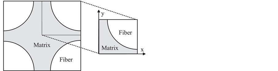
Figure 4. Scheme of a complete 2D RVE for UD carbon fibre composite (left side). 1/4 portion of 2D RVE (right side).
 . (24)
A uniform temperature load is applied to this portion of the unit cell. The coefficients of CTE are finally determined using Equation (22), where the displacements for the calculation of the strains are obtained from the FE solution for the nodes at the boundaries of the unit cell. The advantage of this approach (AP2) is that the desired CTEs are determined by a one calculation of the macroscopic strains of uniform temperature loaded RVE.
The last approach (AP3) for the determination of the effective CTEs is given by
 , (25)
with S* (C*) as the effective compliance (stiffness) tensor. In order to calculate the CTEs, the 1/8 portion of the unit cell is subjected to following boundary conditions: the macroscopic strains are identically equal to zero; the unit cell is subjected to a uniform temperature load DT. The macroscopic stress
 is derived from the calculated microscopic stress s(x) using Equation (2). Finally, the effective CTEs are calculated using Equation (25). However, in order to perform this calculation the effective stiffness (or compliance) tensor should be known. For materials with orthotropic symmetry at least, it is sufficient to determine the components of
 (or
(or ) with i, j = 1, 2, 3 only. This means that three different calculations for the determination of the effective elasticity and Poisson’s ratio moduli have to be performed additionally. The ith column of the effective stiffness tensor is given by
 , (26)
where
 is the jth component of the macroscopic stress due to applied macroscopic strain
 calculated at the reference temperature T0. These additional simulations are the main disadvantage of this approach. However, this approach is very instructive because it indicates clearly that the effective CTEs are related to the effective elastic moduli of the composite. This is the main reason why (semi-)analytical estimates for the effective CTEs use and require the knowledge of reliable (effective) elastic constants of the heterogeneous composite.
7. Conclusions
Three different numerical approaches are employed to compute the effective thermal expansion coefficients of the Dexmet® expanded copper foil 3C7-100FA filled with HexPly® epoxy matrix M21. For the numerical computations, the FEM commercial software ANSYS® is used. The numerical results demonstrate that all developed numerical FEM approaches are accurate and efficient for the analysis of thermo-mechanical properties of heterogeneous composites. The numerically computed longitudinal and transversal effective thermal expansion coefficients of the 3C7-100FA/M21 composite are compared with analytical solutions proposed by Rosen and Hashin and Schapery. The agreement between the numerical and the analytical Rosen and Hashin results is extremely good. The numerical values are within the Schapery analytical bounds as well. However, it should be noted that the numerically (exact) derived values of the effective elastic constants are used for the evaluation of the analytical formulas.
The calculated effective transverse thermal expansion coefficient a2 of the 3C7-100FA/M21 composite is larger than that of the thermal expansion coefficient of the epoxy matrix M21. This result seems to be surprising at first glance, but is has already been mentioned before (see e.g. Kelly [20] and Khare et al. [21] ). The longitudinal thermal expansion coefficient of heterogeneous composite materials is generally small because the inclusions (reinforcements), which usually have a smaller coefficient than that of the polymer matrices, impose a mechanical restrain on the matrix material. The transverse coefficient is generally larger that the longitudinal one. At low inclusion volume fractions it can even be greater than that of the unreinforced polymer matrix, because the matrix, which is prevented from strong expansion in the longitudinal direction, is forced to expand more than usual in the transverse directions. This effect is particularly noticeable at low filler volume fractions for inclusions with high elastic moduli and low expansion coefficients in low-elastic modulus matrices.
An overview of some frequently used analytical and semi-empirical formulas for the effective thermal expansion coefficients of heterogeneous composites is given in addition.
Acknowledgements
The work presented here was partially performed within the framework of the project CARBOSHIELD. Financial support from German BMBF under Contract No. 03X0203B is gratefully acknowledged.
References
- Hashin, Z. (1983) Analysis of Composite Material—A Survey. Journal of Applied Mechanics, 50, 481-505. http://dx.doi.org/10.1115/1.3167081
- Nemat-Nasser, S. and Hor, H. (1999) Micromechanics. Elsevier, Amsterdam.
- Hill, R. (1963) Elastic Properties of Reinforced Solids: Some Theoretical Principles. Journal of the Mechanics and Physics of Solids, 11, 357-372. http://dx.doi.org/10.1016/0022-5096(63)90036-X
- Geers, M., Kouznetseva, V. and Brekelsman, M. (2011) Scale Transition in Solid Mechanics Based on Computational Homogenization. CSIM Lecture Notes, Eindhoven University of Technology, Eindhoven.
- Hyer, M.W. (2009) Stress Analysis of Fiber-Reinforced Composite Materials. DEStech Publications, Inc., Lancaster.
- Voigt, W. (1889) Theoretische Studien über die Elastizit?tsverh?ltnisse der Krystalle. Annalen der Physik, 38, 573-587. http://dx.doi.org/10.1002/andp.18892741206�
- Reuss, A. (1922) Berechnung der Flie?grenze von Kristallen auf Grund der Plastizit?tsbedingung für Einkristalle. Zeitschrift für angewandte Mathematik und Mechanik, 9, 49-58.�
- Turner, P.S. (1946) Thermal Expansion Stresses in Reinforces Plastics. Journal of Research of the National Bureau of Standards, 37, 239-250. http://dx.doi.org/10.6028/jres.037.015
- Levin, V.M. (1967) Thermal Expansion Coefficient of Heterogeneous Materials. Mechanics of Solids, 2, 58-61.
- Hashin, Z. and Shtrikman, S.A. (1962) A Variational Approach to the Theory of the Elastic Behavior of Polycrystals. Journal of the Mechanics and Physics of Solids, 20, 343-352. http://dx.doi.org/10.1016/0022-5096(62)90005-4
- Rosen, B.W. and Hashin, Z. (1970) Effective Thermal Expansion Coefficients and Specific Heat of Composite Materials. International Journal of Engineering, 8, 157-173. http://dx.doi.org/10.1016/0020-7225(70)90066-2
- Schapery, R.A. (1968) Thermal Expansion Coefficient of Composite Materials Based on Energy Principles. Journal of Composite Materials, 2, 380-404. http://dx.doi.org/10.1177/002199836800200308
- Van Fo Fy, G.A. (1966) Elastic Constants and Thermal Expansion of Certain Bodies with Inhomogeneous Regular Structure. Soviet Physics, Doklady, 11, 176-182.
- Budiansky, B. (1970) Thermal and Thermoelastic Properties of Isotropic Composites. Journal of Composite Materials, 4, 286-295. http://dx.doi.org/10.1177/002199837000400301
- Chamberlain, N.J. (1968) Derivation of Expansion Coefficients for a Fibre Reinforced Composites. BAC SON(P) Report 33, British Aircraft Corporation, London.
- Karch, C. and Wulbrand, W. (2013) Thermomechanical Damage of Protected CFRP Structures Caused by Lightning Continuous Currents, SEA2013-20.1. International Conference on Lightning and Static Electricity (ICOLSE), Seattle, 2013, 20.1-20.13.
- Lepetit, B., Escure, C., Guinard, S., Revel, I. and Peres, G. (2011) Thermo-Mechanical Effects Induced by Lightning on Carbon Fiber Composite Materials. International Conference on Lightning and Static Electricity (ICOLSE), Oxford, 2011.
- Karch, C. and Wulbrand, W. (2013) Contributions of Lightning Current Pulses to Mechanical Damage of Protected CFRP Structures: Part 1—Theoretical Survey. CTO/IW-SE-2013-063, EADS, Munich.
- Barbero, E.J. (2011) Introduction to Composite Materials Design. CRC Press, New York.
- Kelly, A. (1989) Conciseencyclopaedia of Composite Materials. Pergamon Press, Oxford.
- Khare, G.A., Chandra, N. and Silvain, J.-F. (2008) Application of Eshelby’s Tensor and Rotation Matrix for the Evaluation of Thermal Transport Properties Composites. Mechanics of Advanced Materials and Structures, 15, 117-129.
- Milton, G.W. (2002) The Theory of Composites. Cambridge University Press, Cambridge. http://dx.doi.org/10.1017/CBO9780511613357
Appendix
Typically the properties of a composite sensitively depend on the topology and microstructure. However, it is sometimes possible to come across exact formulas for effective properties that are universally valid no matter how complicated the microstructure is. In the following, an expression for the effective thermal expansion tensor of a heterogeneous composite consisting of two isotropic constituents is derived and in a second step extended to composites consisting of two anisotropic constituents.
In the linear approximation the thermal expansion is given by the equation
 , (A.1)
where DT = T ‒ T0 is the change in temperature measured from some constant reference temperature T0, while e(x) and s(x) are the microscopic strain and stress fields, and S(x) is the compliance tensor. The average macroscopic strain
 and stress
 fields satisfy a constitutive equation of the same form
 , (A.2)
where S* is the effective compliance tensor and α* is the effective thermal expansion tensor. The stress can be assumed to be a uniform hydrostatic compression (no shear stresses are available)
 , (A.3)
where p is the hydrostatic pressure and I is the identity matrix. For a locally isotropic material the local thermal expansion is given by , and the constitutive equation Equation (A.1) implies that the strain field is given by
 , (A.4)
where K(x) is the local (microscopic) bulk modulus. In the two-phase composite considered the strain field is piecewise constant taking the values
 (A.5)
(A.5)
for each phase i. The requirement that the strain field is uniform
 is, according to above equation, satisfied for any given temperature T when following relation holds
 . (A.6)
Substituting the expression for the average strain and stress fields into Equation (A.2) gives the formula derived by Rosen and Hashin [11] for a composite made from isotropic phases
 . (A.7)
For isotropic composites with a* and K* as the effective bulk modulus the above equation reduces to the formula of Levin [9]
 . (A.8)
In case of anisotropic constituents, the Equation (A.7) can be generalized as follow [22] . The microscopic compliance S(x) and thermal expansion tensor a(x) take constant values in the space of each constituent
 , (A.9)
where c1 and c2 are the characteristic functions
 . (A.10)
Now a solution for a constant stress
 and constant strain field
 (not necessarily proportional to the unit vector I) is sought. The constitutive equations in each phase are given by
 . (A.11)
Finally, the effective anisotropic thermal expansion tensor a* of two-phase composites consisting of anisotropic phases is given by
 . (A.12)
NOTES

1The fourth-rank stiffness tensor has 36 independent components in the most general case. In the linear elastic case only 21 components are independent. The number of independent components can be further reduced by internal material symmetries, i.e. for orthotropic symmetry to 9, for transverse-isotropic to 5, and finally for isotropic symmetry to 2.

2The corresponding effective elasticity moduli and Poisson’s ratios of the 3CU7-100FA/M21 composite are: ,
,
 ,
,
 [GPa] and
 ,
,
 ,
,
 [−]. In order to derive the effective shear moduli macroscopic shearing strains rather than normal uniaxial strains have to be applied. For these calculations the complete symmetrical unit cell of the composite has to be used, see e.g. Reference . The effective shear moduli are:
 ,
,
 ,
,
 [GPa], see Reference .