Open Journal of Civil Engineering
Vol.2 No.2(2012), Article ID:19987,10 pages DOI:10.4236/ojce.2012.22010
Dynamic Analysis of Suspension Bridges and Full Scale Testing
1Bogazici University, Istanbul, Turkey
2Istanbul Aydin University, Istanbul, Turkey
3Civil Engineering, Bogazici University, Istanbul, Turkey
Email: *tezokan@gmail.com
Received January 20, 2012; revised February 18, 2012; accepted March 4, 2012
Keywords: Suspension Bridges; Dynamic Analysis; Tangent Stiffness; Cable Structures; Bridge Testing
ABSTRACT
This paper is concerned with the earthquake analysis of suspension bridges, in which the effects of large deflections are taken into account. The first part of the study deals with an iteration scheme for the nonlinear static analysis of suspension bridges by means of tangent stiffness matrices. The concept of tangent stiffness matrix is then introduced in the frequency equation governing the free vibration of the system. At any equilibrium stage, the vibrations are assumed to take place tangent to the curve representing the force-deflection characteristics of the structure. The bridge is idealized as a three dimensional lumped mass system and subjected to three orthogonal components of earthquake ground motion producing horizontal, vertical and torsional oscillations. By this means a realistic appraisal is achieved for torsional response as well as for the other types of vibration. The modal response spectrum technique is applied to evaluate the seismic loading for the combination of these vibrations. Various numerical examples are introduced in order to demonstrate the method of analysis. The procedure described enables the designer to evaluate the nonlinear dynamic response of suspension bridges in a systematic manner.
1. Introduction
The suspension bridge is a highly nonlinear three dimensional structure. As a consequence, in dynamic studies the governing nonlinear equations of motion are frequently simplified by introducing assumptions which linearize these equations [1]. These simplifying assumptions may however be avoided, and the nonlinear behaviour of the structure may thereby be taken into account in both static and dynamic analyses, by using an iterative solution employing tangent stiffness matrices. The iterative scheme has been successfully applied previously by a number of authors in connection with the static analysis of suspendsion bridges [2-4]. In this paper the same operation is extended to solve the dynamic response problem of suspension bridges, which are idealized as three dimensional lumped mass systems vibrating due to earthquake ground motions. Only geometric nonlinearity is considered; the material is assumed to remain elastic. The method proposed for the nonlinear vibration analysis of suspension bridges involves two distinct steps, as outlined below:
Firstly, under the static action of the dead and live loads the equilibrium configuration and the internal stress resultants of all constituent elements of the structure are first determined through an iteration routine based on the Newton-Raphson method. Secondly, the vibration of any point in the bridge, with respect to the static equilibrium position, is assumed to take place along the tangent to the curve defining the force-deflection characteristics of that point. The natural frequencies and mode shapes of the structure are obtained from a solution of the eigenvalue problem in which the frequency determinant is expressed in terms of the tangent stiffness matrix of the system. Once these fundamental dynamic properties are determined, the response spectrum concept can be used in conjunction with classical modal analysis to evaluate the seismic forces acting on suspension bridges during earthquakes. Details of these two basic steps are given in the following sections.
2. Method of Nonlinear Analysis
For the purpose of clarity, the method of analysis presented in this paper is introduced by reference to the simple nonlinear system shown in Figure 1. A schematic illustration of the iteration process used to obtain the static equilibrium geometry of this example structure is given in Figure 2. Firstly, a linear stiffness analysis is

Figure 1. Sample suspended system.
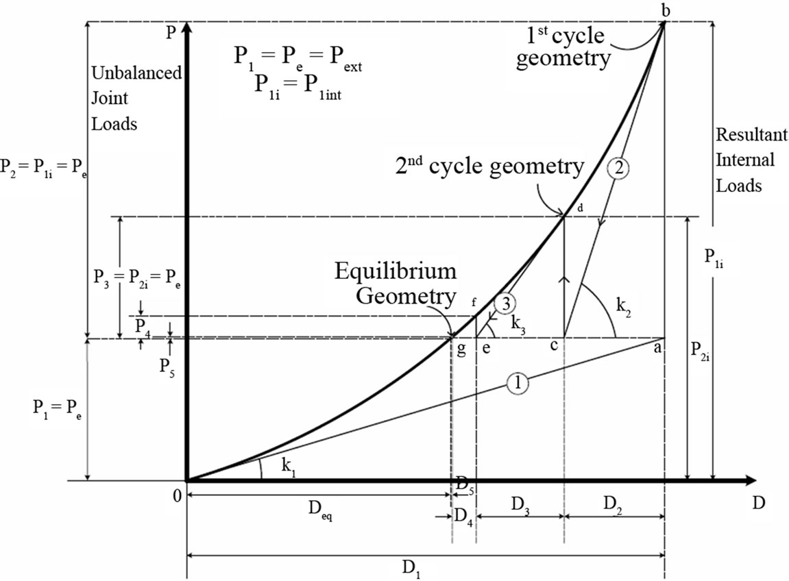
Figure 2. Determination of equilibrium configuration.
performed under the action of the given external load, P1 = Pe, yielding the straight line oa. The slope of this line, K1, is equal to the stiffness of the system in the unloaded position. The joint displacement, D1, obtained from this first linear cycle of analysis is larger than the equilibrium displacement, Deq. Secondly, the internal stress resultants of each member are calculated on the basis of the deformed geometry D1 of the system using the nonlinear expressions of the tangent stiffness matrices given in Appendix . The resultant of the first cycle internal forces, P1i, is not in equilibrium with the external load Pe, as shown in Figure 2. The unbalanced joint load, P2, is
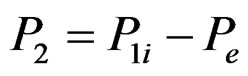 (1)
(1)
In order to eliminate P2, the displacement D1 must be diminished. This is accomplished by loading the joint with a force P2, applied in the direction of the resultant internal joint load P1i, and performing a second linear stiffness analysis of the structure under the action of P2. During this step the original stiffness K1 is replaced by a tangent stiffness, K2, which depends on the loaded member lengths and also on their end deformations and stress resultants in the previous cycle (see Appendix). The forcedeflection characteristic of the structure is now represented by the straight line bc, having slope K2 and leading to a cycle displacement D2, which reduces the initial displacement and brings the system closer to the actual equilibrium configuration. With repeated applications of the above mentioned linear cycles of analyses, the unbalanced joint load is continuously diminished, as may be seen in Figure 2. The tangent stiffness matrix is successively updated after each cycle so as to include the latest geometry and internal stress resultants of the system. At the end of any jth cycle the unbalanced joint load is
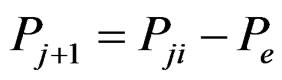 (2)
(2)
and the total joint displacement, Djt , is equal to the algebraic sum of the individual cycle displacements as,
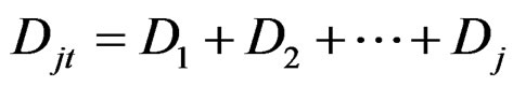 (3)
(3)
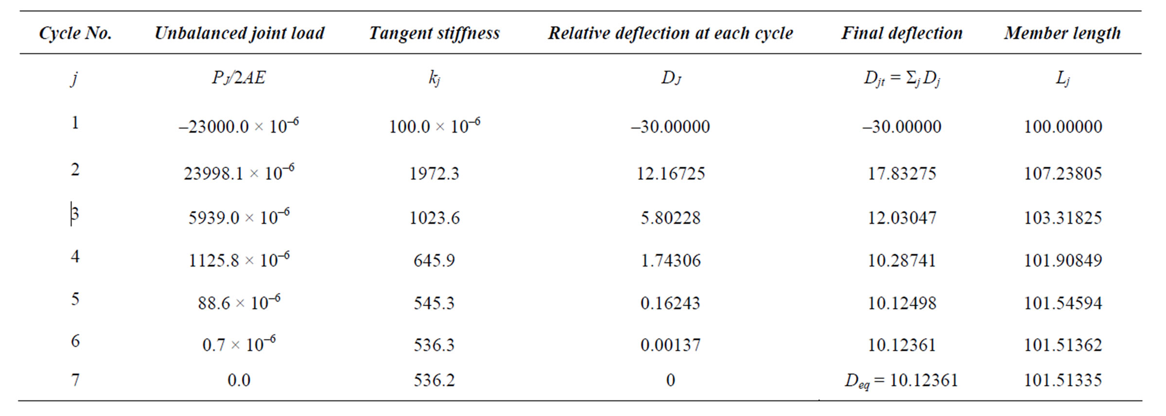
The iterative process is repeated until the unbalanced joint load is reduced to some acceptable value. The above iterative scheme has been applied to the system shown in Figure 1, and the numerical results of each cycle are tabulated in Table 1. Although, seven cycles were required to reach an exact solution, the error in the deflecttion after the fourth cycle was only 1.6%.
3. Equilibrium Configurations
The preceding approach for establishing the equilibrium geometry of nonlinear structures is perfectly general and can be applied without variation to more complicated structures providing that the unbalanced loads are eliminated in every direction at every joint. However, in the case of suspension bridges the entire dead load is carried by the hangers and main cable only. The stiffening girder is assumed to be unstressed and the towers, which carry only an axial load, do not bend under dead load condition. Therefore, the geometry of the suspension bridge available to the designer is usually the dead load equilibrium geometry, and the unloaded lengths of the cables and hangers are unknown. Since these unloaded lengths appear in the tangent stiffness matrices, it is necessary to calculate them before establishing any subsequent geometric configuration as a result of added live loads. The unloaded geometry may be determined from a single cycle of linear analysis under the action of the known dead loads. The unloaded member lengths, L0, may be obtained from Hooke’s Law as
 (4)
(4)
where L = the member length in the known dead load equilibrium configuration, AE = the axial rigidity of the member and Q = the member axial force due to dead loads. With the application of live load the originally unstressed carriage way participates in the overall behaviour of the bridge, which subsequently acquires a new equilibrium geometry, as illustrated in Figure 3. It should be noted that since the carriage way is not stressed under the dead load condition, the unloaded lengths of the members in the carriage girder are available from the known dead load geometry. The number of iteration cycles needed to establish the equilibrium configuration is obviously dependent on the degree of nonlinearity and on
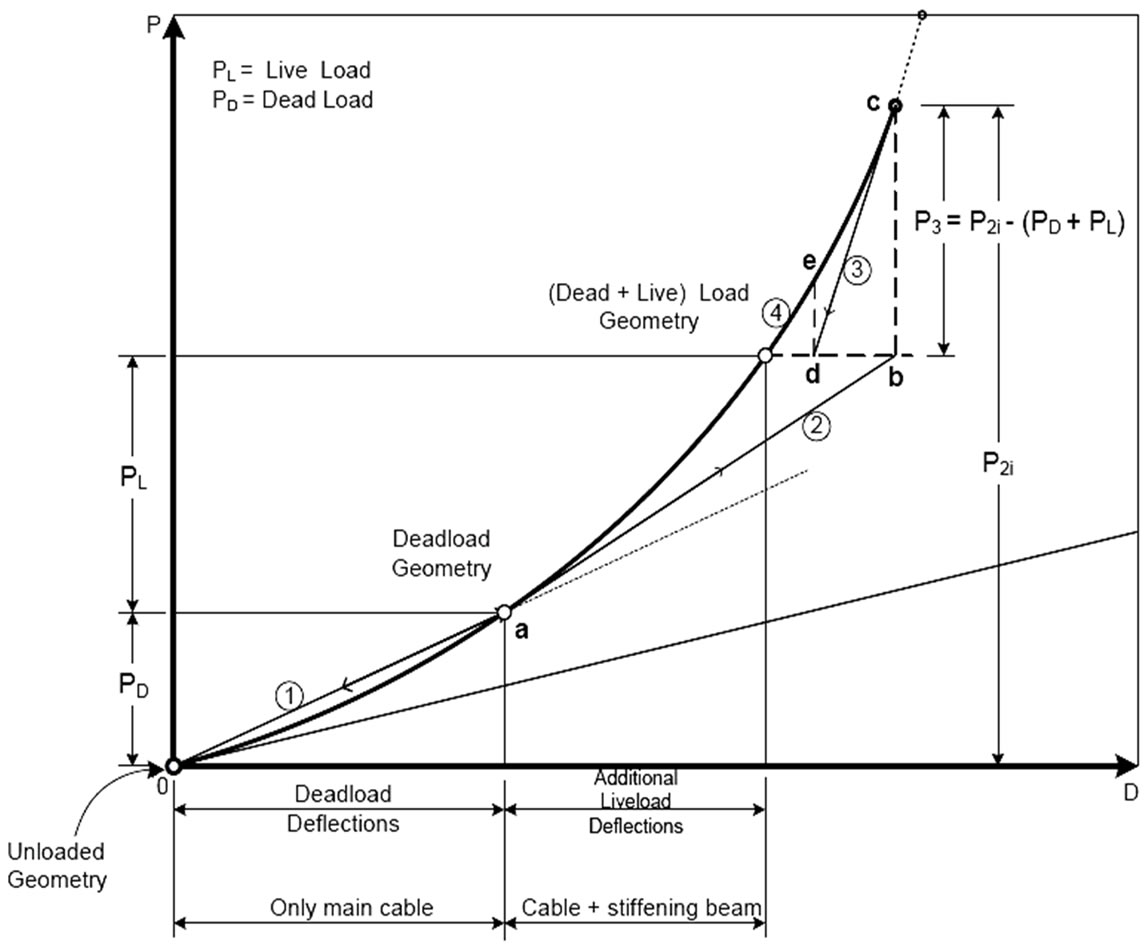
Figure 3. Dead load and live load geometries.
the desired accuracy. In most studies of actual suspension bridges undertaken by the writers, four to six cycles were sufficient to eliminate the unbalanced joint loads to within an accuracy of about 0.3% of the maximum internal stress resultant.
4. Frequency Analysis by Tangent Stiffnesses
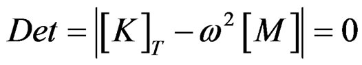
The dynamic analysis of discrete mass structures is a topic which has received extensive treatment in the literature and is well known [5-7]. The nonlinear behaviour of suspension bridges during vibration about any static equilibrium configuration may be accounted for by replacing the linear stiffness matrix of the system, [K]o, by a tangent stiffness matrix, [K]T = [K]o + [K]g . This is equivalent to assuming that at any equilibrium stage the vibration of any point in the bridge takes place along the tangent to the curve representing the force-deflection characteristics of the point. This idea of tangential vibration is illustrated in Figure 4. Accordingly, the frequency determinant becomes
 (5)
(5)
where, M = mass matrix, and ω = the natural frequency of the system in any one of its normal modes. [K]T depends on the strains and the internal forces developed in the members at the static equilibrium position. The eigenvalues, ω, as well as the eigenvectors, can be obtained from a solution of Equation (5) using routine computer programs. The concept of tangential vibration may be simply illustrated by application of the single degree of freedom suspended system shown in Figure 5. This structure is considered to be vibrating freely about static equilibrium Position 3, corresponding to some dead and live load combination. The dynamic displacement of the system from the equilibrium position is defined by z, measured positive downward. This deformation is repre-
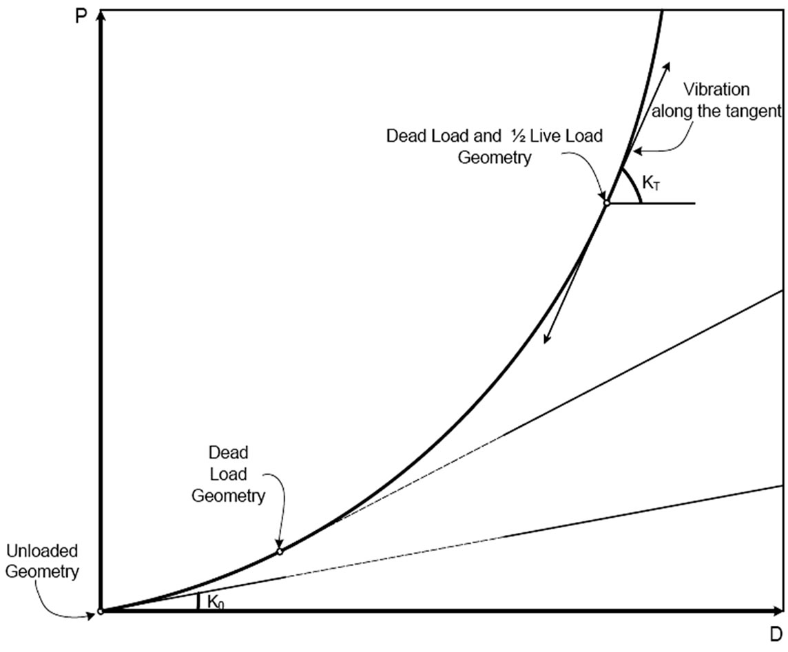
Figure 4. Vibration along the tangent line.
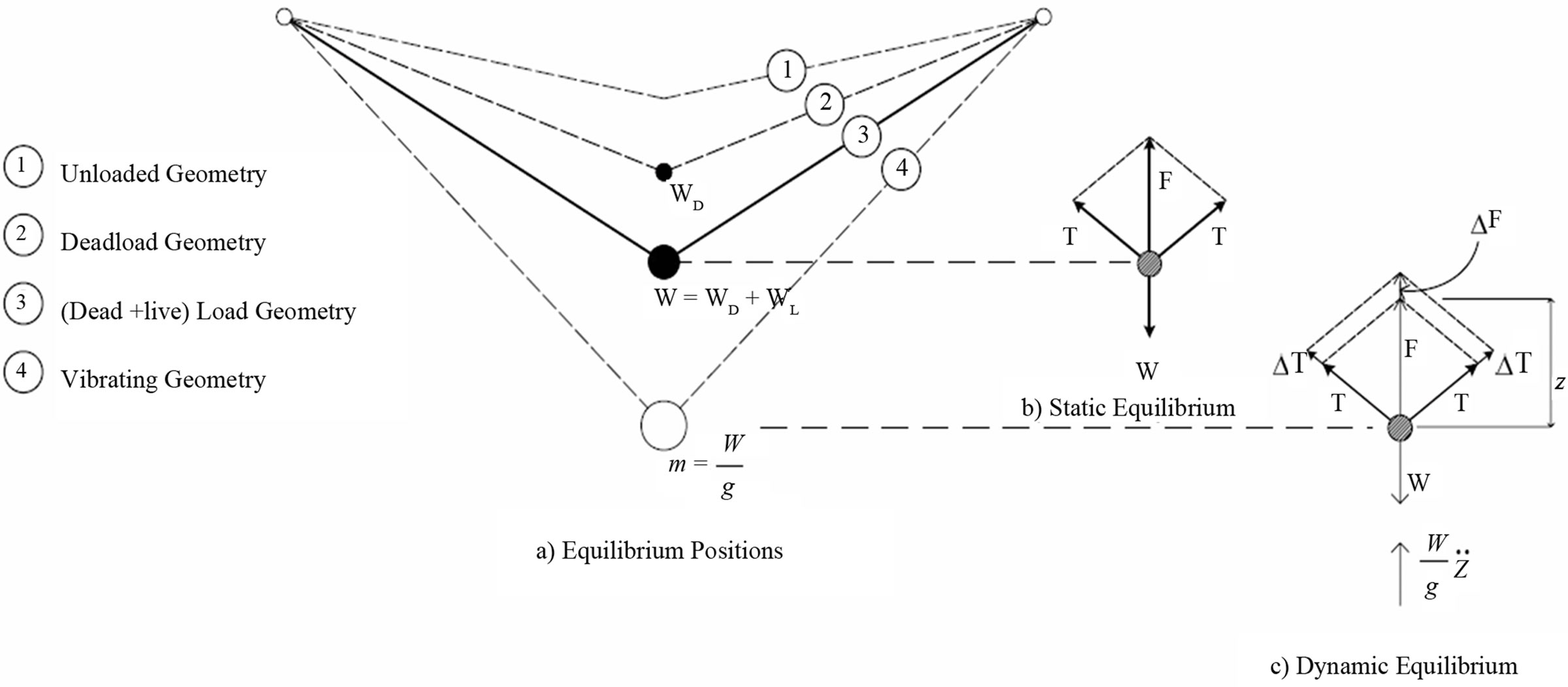
Figure 5. Vibration of a nonlinear suspended system.
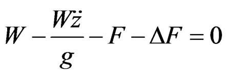
sented by Position 4. Then, in accordance with D’Alembert’s principle, from Figure 5(c),
 (6)
(6)
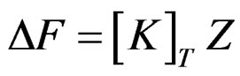
From statics, the resultant of the cable forces, F, is equal and opposite to the sum of the dead and live loads, W. When the system is translated by the amount z into Position 4 the resultant of the cable forces is increased by an increment ΔF, in order to maintain equilibrium. This increment is simply the product of the tangent stiffness of the cables, KT, and the displacement z. That is,
 (7)
(7)
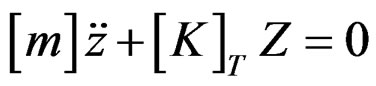
where KT is defined as the force required to deform the structure through a unit vertical displacement, measured with respect to the dead plus live load equilibrium geometry under consideration. With the substitution of F = W, m = W/g and ΔF = KT z, Equation (6) is reduced to
 (8)
(8)
The response of the linear multidegree of freedom system can be described in terms of a combination of a number of equivalent single degree of freedom systems whose behaviours are governed by a set of independent equations of the above form. For the nonlinear system, in which tangential vibrations are contemplated, the dynamic response can therefore be obtained by direct application of the standard modal superposition technique, once the nonlinearity of the structure has been taken into account inside the stiffness matrix and Equation (5) has been solved. The modal superposition approach has previously been applied to suspension bridges [1,8], but the nonlinearity of the structure was not taken into account inside the stiffness matrix.
5. Idealization of the Bridge
Depending on the memory capacity of the computer available, the suspension bridge may be idealized as a plane or space frame composed of a series of straight line elements. While the plane frame idealization may be used for the study of the response to vertical and longitudinal ground motions, the three dimensional idealization is desirable for a realistic investigation of the torsional and lateral vibrations of the deck due to ground motion perpendicular to the deck centerline. The main cable and hangers are considered as pure axial force members of constant cross-section, while the deck is assumed to be composed of beam-column elements between hangers. Loads are considered to act at the nodal points only. Since the stiffness matrix approach is quite general, it is not necessary to resort to any other simplifying assumptions. The influence of hanger extensions, cable point loads, degree of fixity at the tower base, stability coefficients due to compressive forces in the bending of tower continuity of the deck across the towers, and variations in moments of inertia can easily be taken into account [9,10].
In the case of a three dimensional idealization, all three rotations and the horizontal translations perpendicular to the bridge centerline have been suppressed at the cable - hanger junctions in order to prevent singularity in the stiffness matrix. This reduces the total number of degrees of freedom of the system. Further, distributed consistent mass matrices, rather than the lumped masses, have been used for each structural element during the full scale 3D-analyses.
6. Primary and Secondary Degrees of Freedom
The joints of a vibrating structure normally have more degrees of freedom than the number of directions along which the vibrations take place. For example, the joints of the cables and hangers are not considered to vibrate in the rotational degrees of freedom. To distinguish between the vibrating and non-vibrating directions, the degrees of freedom are classified into two groups as, Primary (P) and secondary (S) degrees of freedom.
The master stiffness matrix generated for the system contains both primary and secondary degrees of freedom and is therefore of higher order than the size of the mass matrix of Equation (5) In order to make the matrices compatible, the master tangent stiffness matrix size is reduced by eliminating the secondary degrees of freedom (S), through a matrix partitioning process [7]. Alternatively, there will be no necessity for matrix portitioning, if the rotary moments of inertia are supplied for flexural members [11].
7. Types of Vibration
An earthquake may excite a suspension bridge in any one or a combination of the following three types of vibration. At any rate, a full 3-D modeling and analysis of the bridge will already accommodate all these three types of vibration and will output them in various mode shapes:
1) Torsional vibration of the bridge deck, coupled with a lateral vibration of the towers, is due to horizontal ground motion perpendicular to the centerline of the bridge. The torsional vibration is essentially a combination of the vertical and lateral motion of the bridge deck. Such vibrations may also be developed due to lateral wind loading.
2) Horizontal and vertical vibrations of the bridge deck, coupled with horizontal vibrations of the towers, are due to horizontal ground motion parallel to the centerline of the bridge.
3) Vertical vibrations of the bridge deck, coupled with a horizontal (in longitudinal direction) vibration of the towers, are due to vertical ground motion.
In all cases, vertical (axial) vibrations of the towers and also longitudinal (axial) vibrations of the bridge deck may be neglected, since their effects are relatively small. These three types of vibrations should be taken into account when performing an earthquake analysis of 3Dsuspendsion bridges. Different aspects of this problem have been discussed in the literature for suspension bridges [12-19] and also for cable stayed bridges [20,21].
8. Numerical Examples
The procedures discussed in the preceding sections will now be demonstrated by application to two example structures. The idealized N-S component of the 1940 El Centro earthquake spectrum [5] was used in the dynamic analysis of both structures; the spectrum values were multiplied by two-thirds when considering vertical excitation. The bridges were considered to have 1% of critical damping in all modes, and the tower and anchorage supports were assumed to be subjected to the same ground motion. Although, the capacity of the program was sufficient to handle full scale suspension bridges, smaller hypothetical structures were selected for sake of simplicity and clarity of presentation.
1) Example 1.
A hypothetical suspension bridge was idealized as a 2D lumped mass system as shown in Figure 6 and subjected to vertical ground motion only. The structural member properties of the bridge are summarized in Table 2. As discussed in Section 7, this excitation produced
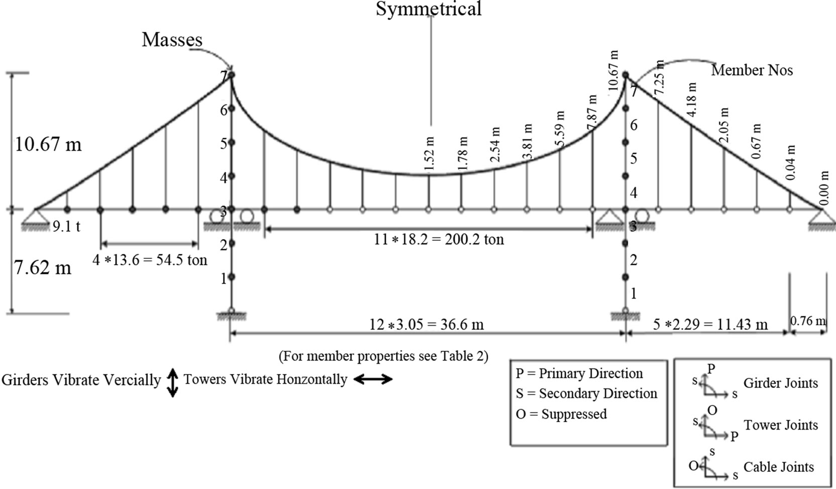
Figure 6. Idealised suspension bridge (Example 1).
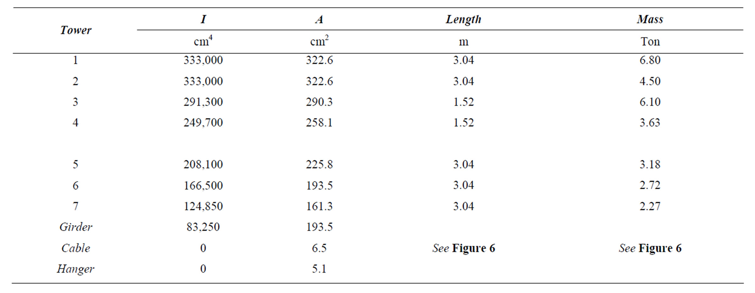
Table 2. Member properties of example 1 (E = 210,000 MPa).
vertical vibration of the deck and horizontal vibration of the towers. The primary (P) and secondary (S) degrees of freedom corresponding to the vertical ground motion are also shown in Figure 6 for a typical cable, girder and tower joint. The static equilibrium position about which the bridge was assumed to vibrate was taken as the dead, plus one-half live load configuration, which was established by the iteration scheme outlined in Section 2 through Section 6. The mode shapes and natural periods for the first ten modes of vibration are illustrated in Figure 7.
2) Example 2.
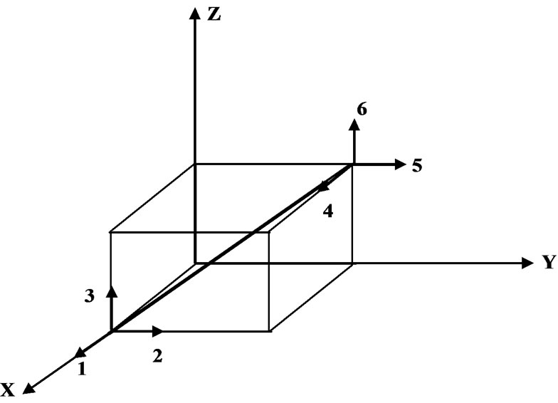
In order to obtain a realistic appraisal of the dynamic response of suspension bridges, especially towards lateral ground motion, a three dimensional idealization of the structure is desirable. The unloaded and deformed shapes of a plane frame member are shown in Figure 9, while the deformation numbers of a 3D-truss and frame member are shown in Figure 10. For the purpose of illustration, the centre span of the preceding example was idealized into the twenty eight lumped mass system shown in Figure 8. The member properties are listed in Table 3. The bridge was subjected, non-concurrently, to the three types of vibrations described in Section 7. The geometry supplied in Figure 8 was assumed to be the equilibrium geometry about which the vibrations occurred. The lumped masses of the bridge deck were assumed to have both vertical and horizontal motions, allowing the investtigation of torsional vibrations.
The natural periods, participation factors, spectral displacements and the mode shapes for the first ten modes of vibration, are given in Table 4. The horizontal and vertical mode shapes are of the same form as those shown with the preceding example, Figure 7. Mode 6 and Mode 8 indicate the presence of a torsional oscillation of the bridge deck. This potentially destructive vibration, which has caused real suspension bridge failures,
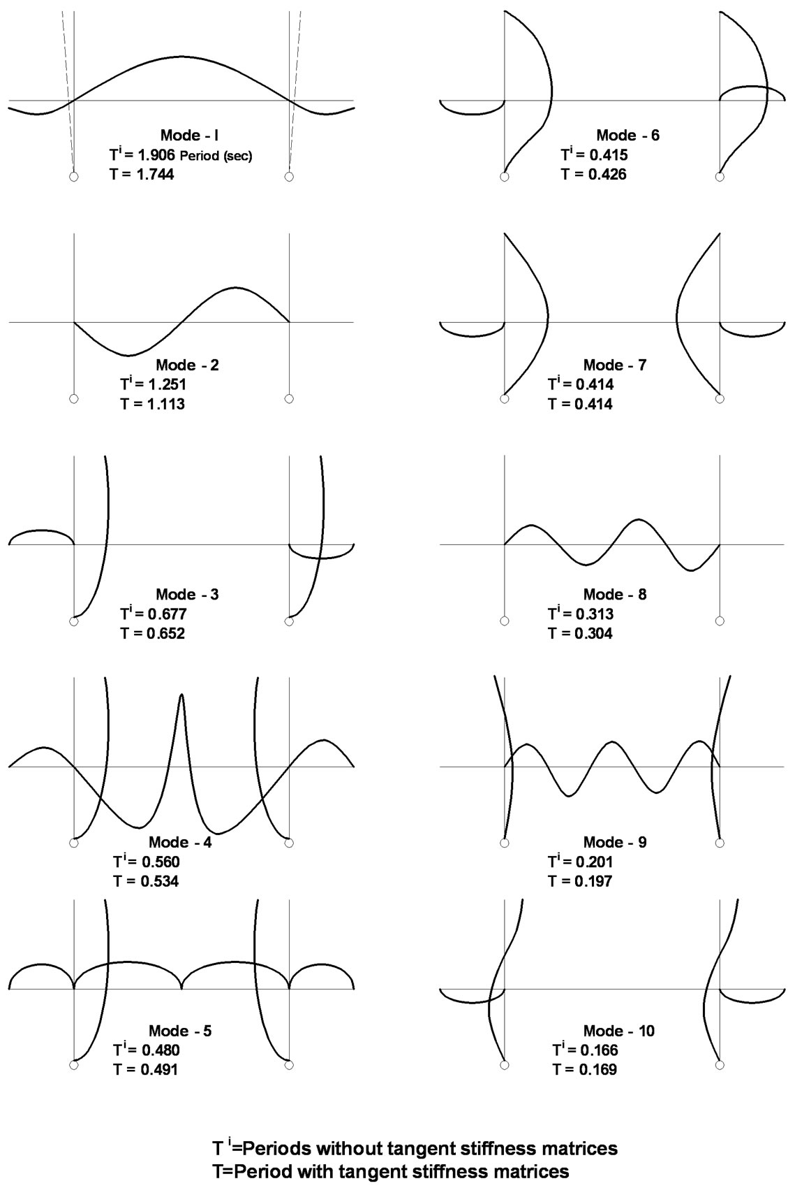
Figure 7. Mode shapes of Example 1.
such as Tacoma Narrows Bridge, in Washington, USA on November 08, 1940, emphasizes the usefulness of the three dimensional idealization. Only two of the first ten modes of vibration were of a torsional character. It is possible that higher torsional modes would have a significant influence on the maximum response.
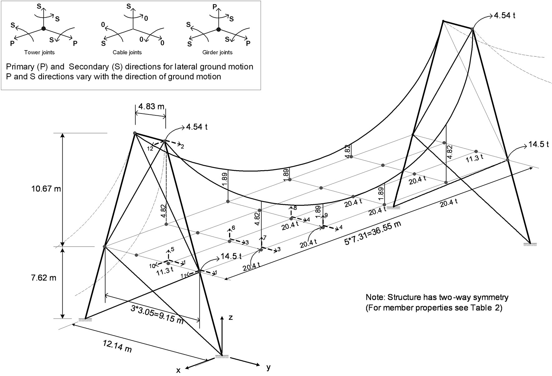
Figure 8. Idealised suspension bridge (example 2).

Figure 9. Unloaded and deformed members.
3) Example 3.
A new suspension bridge named Chanakkale Ataturk Bridge is proposed for the Chanakkale Strait at a total length of 2200 meters [22]. It is believed that this bridge will boost the economical ties between Turkey and the European Countries, will enhance tourism all along the western and southern coastal regions of Turkey. A submerged floating tunnel is also proposed by Tezcan et al. [23] for the Gibraltar crossing between Morocco and Spain. The total length of this floating tunnel is envisaged to be 14.5 kilometers of which 12.2 kilometers will be 100 meter under the sea. The discussion for the numerical analyses of these two long span crossings is too lengthy to be included within the framework of this paper.
 (a)
(a)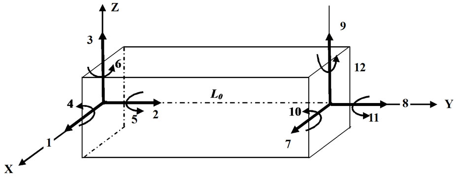 (b)
(b)
Figure 10. 3D-truss and frame members.
9. Full Scale Bridge Testing
The ambient and the forced vibration test results of the Istanbul Bogazici Bridge, are the successful examples for the correlation of analytical and experimental studies. Just a month before the opening of the Istanbul Bogazici Bridge (Figure 11) to traffic early in October 1973, a series of insitu experimental studies have been conducted, under the general supervision of the writers, as follows [24]:
1) Strain gauge readings were taken at a number of locations on the orthotropic deck, towers and hangers,
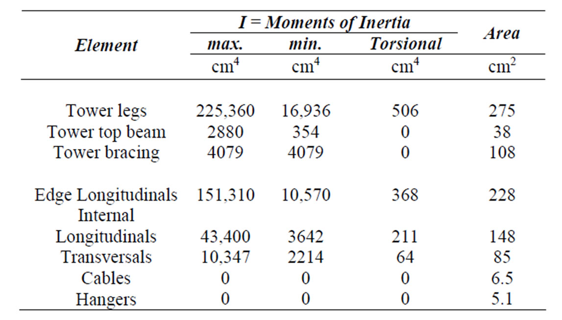
Table 3. Member properties of example 2 (E = 210,000 MPa).
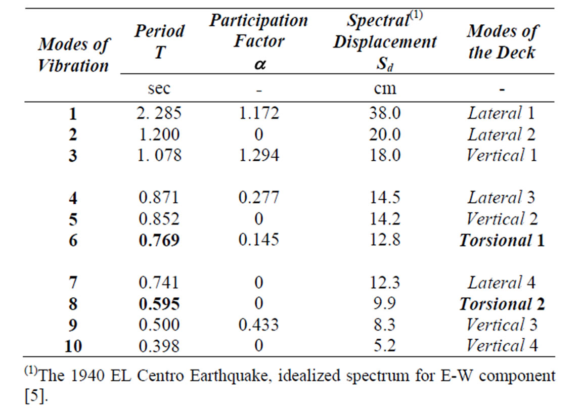
Table 4. Response analysis of the suspension bridge, example 2.
(1)The 1940 EL Centro Earthquake, idealized spectrum for E-W component [5].
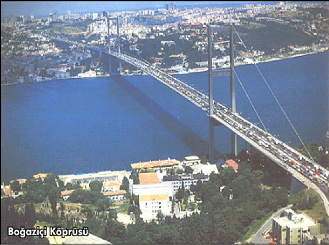
Figure 11. A general view of Istanbul Bogazici Bridge.
when the carriage ways between the two towers were loaded with heavy trucks up to three fourths of the bridge capacity. The deflections of the deck, under this particular loading, were also determined by means of precise leveling. The maximum centerline deflection was measured to be 0.96 m, as verified by the 3D nonlinear analytical calculations described above.
2) Three different sets of seismometers a) by İstanbul Kandilli Observatory team; b) by the team of seismologists from the Earthquake Engineering Institute of Skopje and c) by Mr. Alkut Aytun, a Turkish seismologist, have been installed over the deck and the south tower in order to record the ambient wind vibrations of the bridge. The inversed fourier transform technique has been used to determine the fundamental periods of vibration. Locations of seismometers and the 2D—mathematical model of the bridge are shown in Figure 12. The results of the ambient vibration tests are very close to those reported earlier by Brownjohn et al. [25].
3) Two Synchronised twin shakers of the type GSV- 100 Teledyne, USA supplied by the Skopje Institute were welded at midspan and quarterspan points of the deck as shown in Figure 13, and the forced vibrations were recorded. The fundamental periods of vibration for a variety of relatively higher modes were determined together with the values of b = critical damping ratio. Most of the results and key parameters obtained from these tests, including those obtained from the wind tunnel tests at the National Physical Laboratories, Teddington, England are listed in Table 5.
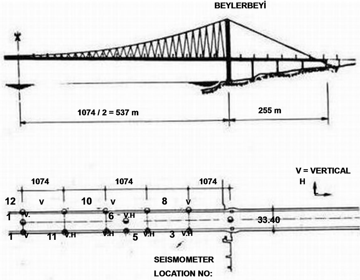
Figure 12. Location of seismometers.
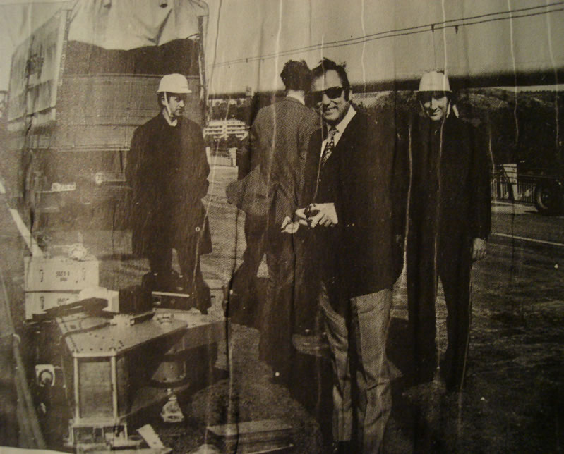
Figure 13. Shakers welded onto the deck by Skopje Institute.
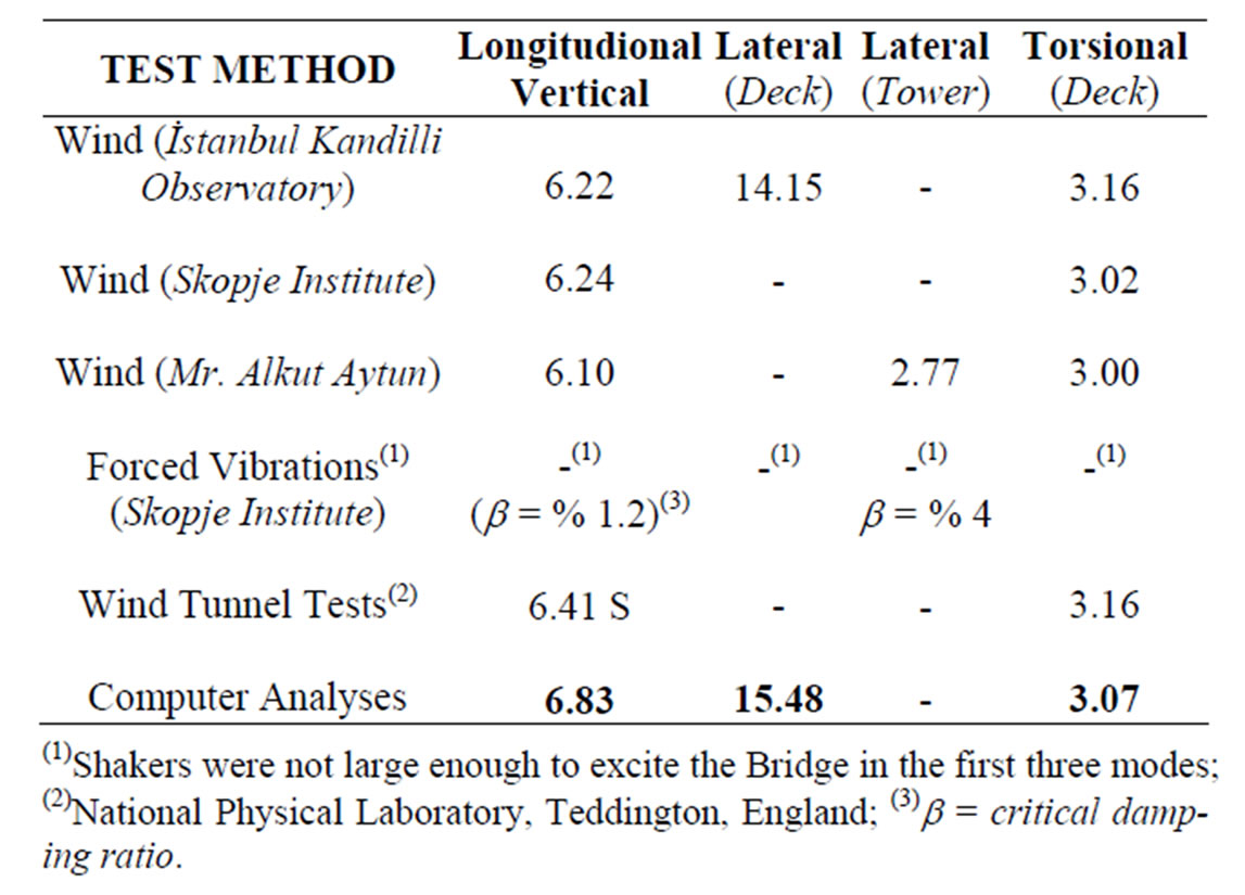
Table 5. Results of ambient and forced vibration tests, Istanbul Bogazici Bridge, (sec).
(1)Shakers were not large enough to excite the Bridge in the first three modes; (2)National Physical Laboratory, Teddington, England; (3)b = critical damping ratio.
10. Conclusions
1) The concept of tangent stiffness matrix, used in conjunction with the standard modal superposition method, provides a systematic approach to the nonlinear dynamic analysis of suspension bridges.
2) For a realistic evaluation of the overall dynamic response of a suspension bridge, a three dimensional idealization is desirable. Such an idealization permits a study of the torsional oscillations of the bridge deck. In fact, significant vibrations of this type were observed due to earthquake ground motion perpendicular to the bridge centerline.
3) The general procedures described in this paper may supply useful information in the study of the aerodynamics of suspension bridges.
REFERENCES
- I. Konishi and Y. Yamada, “Earthquake Responses of a Long Span Suspension Bridge,” Proceedings of the Second World Conference on Earthquake Engineering, Tokyo, Vol. 2, 1960, pp. 863-875.
- D. M. Brotton, “A General Computer Programme for the Solution of Suspension Brdige Problems,” Structural Engineer, Vol. 44, No. 5, 1966, pp. 161-167.
- S. A. Saafan, “Theoretical Analysis of Suspension Bridges,” Journal of the Structural Division, Vol. 92, No. ST4, 1966.
- S. S. Tezcan, “Stiffness Analysis of Suspension Bridges by Iteration,” Proceedings, Symposium on Suspension Bridges, Laboratorio Nacional de Engenharia Civil, Avenue Du Brasil, Lisbon, November 1966.
- J. A. Blume, N. M. Newmark and L. H. Corning, “Design of Multistorey Reinforced Concrete Buildings for Earthquake Motions,” Portland Cement Association, Chicago, 1961, p. 245.
- G. W. Housner, “Behaviour of Structures during Earthquakes,” Journal of the Engineering Mechanics Division, Vol. 85, No. SM4, 1953, pp. 109-129.
- W. G. Hurty and M. F. Rubinstein, “Dynamics of Structures,” Prentice-Hall Inc., New York, 1964.
- I. Konishi and Y. Yamada, “Earthquake Response and Earthquake Resistant Design of Long Span Suspension Bridges,” Proceedings of the 3rd World Conference on Earthquake Engineerings, Vol. 3, 2004, pp. 312-323.
- R. K. Livesley and B. D. Chandler, “Stability Functions for Structural Frameworks,” Manchester University Press, Manchester, 1956.
- M. J. Turner, E. H. Dill, H. C. Martin and R. J. Melosh, “Large Deflections of Structures Subjected to Heating and External Loads,” Journal of the Aero-Space Sciences, Vol. 27, No. 2, 1960, pp. 97-106.
- S. S. Tezcan, “Discussion of Numerical Solution of Nonlinear Structures,” Journal of the Structural Division, Vol. 94, No. ST6, 1968, pp. 1613-1623.
- D. B. Steinman, “Modes and Natural Frequencies of Suspension Bridge Oscillations,” Journal of the Franklin Institute, Philadelphia, Vol. 3, No. 4, 1959, pp. 148-174. doi:10.1016/S0016-0032(59)90395-3
- A. Hirai, T. Okumura, M. Ito and N. Narita, “Lateral Stability of a Suspension Bridge Subjected to Foundation Motion,” Proceedings of the 2nd World Conference on Earthquake Engineering, Tokyo, 11-18 July 1960, pp. 931-945.
- K. Kubo, “Aseismicity of Suspension Bridges Forced to Vibrate Longitudinally,” Proceedings of the 2nd World Conference on Earthquake Engineering, Tokyo, 11-18 July 1960, pp. 913-929.
- S. S. Tezcan, “Computer Analysis of Plane and Space Structures,” Journal of the Structural Division, Vol. 92, No. ST2, 1966, pp. 143-174.
- M. Zribi, N. B. Almutairi and R. M. Abdel, “Control of Vibrations Due to Moving Loads on Suspension Bridges,” Journal of Engineering Mechanics, Vol. 132, No. 6, 2006, pp. 659-670. doi:10.1061/(ASCE)0733-9399(2006)132:6(659)
- N. P. Jones and C. A. Spartz, “Structural Damping Estimation for Long-Span Bridges,” Journal of Engineering Mechanics, Vol. 116, No. 11, 1991, pp. 2414-2433. doi:10.1061/(ASCE)0733-9399(1990)116:11(2414)
- R. S. Harichandran, A. Hawwari and B. N. Sweidan, “Response of Long-Span Bridges to Spatially Varying Ground Motion,” Journal of Structural Engineering, Vol. 122, No. 5, 1991, pp. 476-484. doi:10.1061/(ASCE)0733-9445(1996)122:5(476)
- A. M. Abdel-Ghaffar, S. F. Masri and A. S. M. Niazy, “Seismic Performance Evaluation of Suspension Bridges,” Proceedings of the 10th World Conference on Earthquake Engineering, Madrid, 19-24 July 1992, pp. 4845-4850.
- J. F. Fleming and E. A. Egeseli, “Dynamic Behavior of a Cable-Stayed Bridge,” Earthquake Engineering and Structural Dynamics, Vol. 8, No. 1, 1980, pp. 1-16. doi:10.1002/eqe.4290080102
- A. M. Abdel-Ghaffar and A. S. Nazmy, “3-D Nonlinear Seismic Behavior of Cable-Stayed Bridges,” Journal of the Structural Division, Vol. 117, No. 11, 1991, pp. 3456- 3476. doi:10.1061/(ASCE)0733-9445(1991)117:11(3456)
- S. S. Tezcan and E. Arıoğlu, “Chanakkale Ataturk Bridge,” Proceedings of the 3rd Symposium on Strait Crossings, Norwegian Road Research Laboratory, Alesund, 12-15 June 1994, pp. 21-35.
- S. S. Tezcan and K. Kaptan, “A Submerged Floating Tunnel Proposal for the Gibraltar Crossing,” Proceedings, 4th Inernational Congress on the Gibraltar Straits Fixed Link, Seville, Vol. 3, 16-18 May 1995, pp. 347-356.
- S. S. Tezcan, M. İpek, J. Petrovski, T. Paskalov and T. Durgunoglu, “Ambient and Forced Vibration Survey of Istanbul Bogazici Suspension Bridge,” Proceedings of the 5th European Conference on Earthquake Engineering, Istanbul, Chapter 9, September 1975.
- J. M. W. Brownjohn, A. A. Dumanoğlu, R. T. Severn and A. Blakeborough, “Ambient Vibration Survey of the Bosphorus Suspension Bridge,” Earthquake Engineering and Structural Dynamics, Vol. 18, No. 2, 1989, pp. 263- 283. doi:10.1002/eqe.4290180210