Open Journal of Biophysics
Vol.2 No.1(2012), Article ID:17115,8 pages DOI:10.4236/ojbiphy.2012.21003
A Neighborhood Method for Statistical Analysis of fMRI Data
1Department of Mathematical Sciences, Korea Advanced Institute of Science and Technology,
Daejeon, Korea
2Theoretical Biology and Biophysics, Los Alamos National Laboratory, Los Alamos, USA
Email: fayyazm3@kaist.ac.kr, gullah@lanl.gov, sung-ho.kim@kaist.edu
Received October 28, 2011; November 30, 2011; accepted December 7, 2011
Keywords: Statistical Parametric Mapping; Autoregressive Model; Initial Values; ROC Curve; GLM; Regions of Interest
ABSTRACT
In an effort to cope with the fact that functional magnetic resonance imaging (fMRI) data are spatiotemporally correlated, we propose a novel statistical method with a view to improve the detection of brain regions with increased neuronal activity in fMRI. In this method, we make use of information from neighboring voxels of a voxel, for estimation at the voxel. We examined performance of the method against the statistical parametric mapping (SPM) method using both simulated and real data. The proposed method is shown to be considerably better than the SPM in the context of receiver operating characteristics (ROC) curves.
1. Introduction
Functional magnetic resonance imaging data analysis are evolving quickly in a fast growing community, because of the excellent temporal and spatial resolution of these data and the innocuous aspect of their acquisition in human brains. One of the major objectives of fMRI studies is to determine which areas of the brain are activated in response to a stimulus or task. Functional imaging data are based on the principles of magnetic resonance and the fact that increases in neural activity are accompanied by changes in regional cerebral blood flow (rCBF) and blood oxygenation. This blood oxygenation level dependent (BOLD) effect is the basis for most of the fMRI studies for mapping patterns of activation in the working human brain. Lueck et al. [1] and Friston et al. [2] are among the first to develop a statistical parametric mapping package (SPM) by using MATLAB (programming language) to map patterns of activation based on a fMRI data, which are available in the public domain (www.fil.ion.ucl.ac.uk/spm).
fMRI data have a time sampling that allows for a precise estimation of the neuronal response to various experimental conditions. SPM is typically analyzed fMRI data to various conditions with a massively univariate approach, where a univariate general linear model (GLM) is fit independently at every voxel. In SPM, there is a major problem for fitting the univariate GLM, the successive fMRI scans of every voxel of the brain are not independent or spatiotemporally correlated. A solution to this problem was given by Worsley and Friston [3,4] which provided a general framework for the spatiotemporally correlated fMRI scans. In their framework, they estimate the error covariance matrix 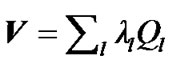 of size s × s from the fMRI data, by employing the restricted maximum likelihood estimate method (ReMLE) [5]. They used
 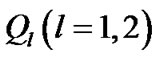 constraints in the form of
 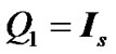 and
and 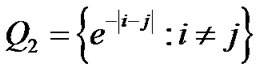 where
where  is an identity of size s (total number of time points) of fMRI data,
  and
and  In the V matrix, they estimate global hyperparameters
  ( error variance components ) from the autoregressive model ( AR(1) + wn ) based on pooled data from all the interested voxels. They used this estimated error covariance matrix
  in SPM package in the form of
  to make independent successive fMRI scans of every voxel of the whole brain. Finally, they used this independent fMRI data for fitting the GLM of every voxel of the brain to get SPMs or activity map.
The fMRI data are temporally correlated or autocorrelated and functional imaging data have some spatial correlation. This spatial correlation is further enhanced by some operations with the analysis of SPM such as smoothing and re-slicing fMRI data, and also, fMRI data of low resolution from an individual voxel will contain some signal from the tissue around that voxel. This spatiotemporal autocorrelation Valdes-Sosa [6] has led us to propose a method in which we incorporate estimation results at neighboring voxels of a voxel, v say, in the estimation at voxel v. This proposed method is shown to improve the detection of brain regions with increased neuronal activity which is statistically more powerful as compared to the ReMLE approach of SPM.
2. The Proposed Method
We propose regularizing the autocorrelations based on neighboring voxel as described in details in the next Section (2.1). In practice the estimated autocorrelation parameters vary considerably about their true values. Even when no correlation is present, it is well known that the standard deviation of the sample autocorrelation ϱ is about
  by [7]. Some method of regularization that reduces this variability seems desirable. Purdon et al. [8] achieve this by spatial smoothing of the likelihood before estimating the autocorrelation parameters.
We analyzed the fMRI data with regard to temporal correlation, the SPM does not consider any relationship among voxels to make independent data for fitting GLM. For the efficient analysis, SPM estimates a global value of ϱ by using model AR(1) + wn based on pooling the sample autocorrelations of the fMRI raw data that create bias result. In the fMRI data set, there were variations in the strength of correlation and SPM’s global ϱ cannot adapt to these local changes. This supports the need for local autocorrelation modeling based on neighboring voxels information in order to ensure unbiased result in the form of accurate detection of activation, p-values and valid inferences at every voxel. The estimates of parameters and the variance
  of the white noise of model (3) of all the voxels of a middle slice from real fMRI data of Section 3.3 are shown in Figure 1. Moreover the variations in the estimated variance
  values of all the voxel of a same slice in Figure 2 can also be clearly observe in the form of bird-view. Due to these variation of the parameters and incorporates the spatial correlation between neighboring voxels, we propose an accurate pre-whitening strategy with estimation made at every voxel in the brain. We will call this strategy a neighborhood method (NH). We compare our approach by modifying the SPM code to functional imaging with the ReMLE method which has been established by Friston et al. [4] and Worsley et al. [5].
2.1. Neighborhood Algorithm
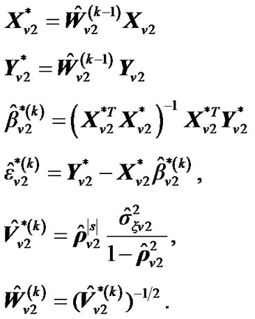
In our method, we denote an fMRI data set consisting of s time points or scans at n voxels as the s × n matrix Y. In mass-univariate GLM model [Friston et al. 1995], these data are explained in terms of a s × m design matrix X, containing the values of m regressors at s time points, and a m × n matrix of regression coefficients β, containing m regression coefficients at each of the n voxels. The model is written

Figure 1. Estimated variance  and
and  (histogram) values of model (3) of all the voxels of a middle slice of real data. The x-axis represents voxel labels (top panel) and thê values (bottom panel). The estimates are from the NH method.
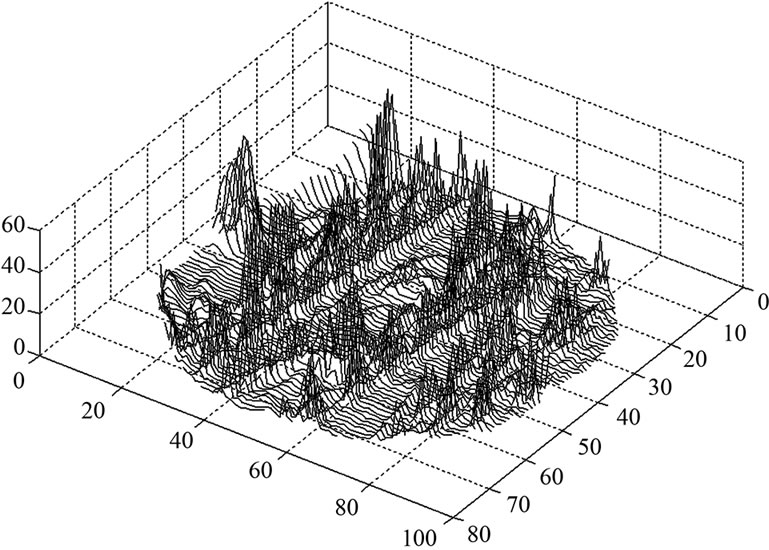
Figure 2. A bird-view of the estimated variance  values of model (3) of all the voxels of a middle slice of real data.
 (1)
(1)
where  is a
is a  error matrix.
1) The GLM of the variable Y at voxel  from n voxels is given by
 (2)
(2)
where  is error covariance matrix.
2) Estimate the values,  where
where 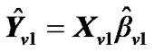 and regression coefficient
  i.e.,
i.e.,
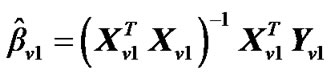 from model (2).
3) Obtain  by using the following simplest model of autocorrelation AR(1) proposed by Bullmore et al. [9] and [10-13].
 (3)
(3)
Where ,
,  is a coefficient of the model and
  is a square matrix whose
  th entry is
 ,
, . i.e.

In the model (3) scans are equally spaced in time and the errors from previous time point,  , are mixed up with a white noise
  into the error of the current time point,
 .
.
4) Calculate the error covariance matrix  as
as . Multiply the general linear model (2) by
 :
:
 (4)
(4)
where ,
,  ,
,  , and regression coefficient
  is then estimated as
 (5)
(5)
a) For a neighboring voxel  of
of , set initial values of the estimates as:
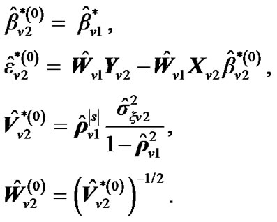
where  is computed based on
  by using model (3).
b) Repeat updating ,
,  and
and  until convergence takes place (e.g.,
 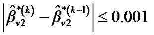 ,
,  and
and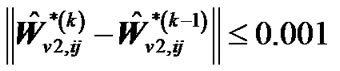 ,
,
c) If a voxel  has more than one voxels where estimation is already made, then we take averages of the estimates from the neighboring voxels for the initial values of the parameters
 ,
, , V, and W. In other words, the right-hand sides of the equations in step 4a are replaced with the corresponding averages of the estimates.
5) Apply step 4 to all the voxels of the brain that are involved in the data.
6) Finally, to detect the effect or activity in terms of optimal  from step (4b), we test the null hypothesis that the effect is zero for every voxel of the brain. An effect of interest, such as a difference between stimuli, can be specified by
 , where C is a row-vector of contrast of m conditions. It is estimated by
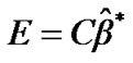
with standard deviation 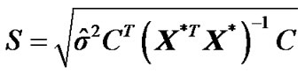 by using estimated error covariance matrix
 . The test statistic is the T-statistic
 (6)
(6)
which is an exactly t-distribution because S is a square root of  distribution with
  degrees of freedom (p is number of parameters ) whereas Worsley and Friston [3] used Satterthwaite approximation [14] for T-statistic and effective degrees of freedom in SPM because in their ReMLE method denominator of T is not a square root of
  distribution.
3. Experimental Results
3.1. Simulated fMRI Data
In order to evaluate our proposed method, we generated a Gaussian artificial signals in a 4-D fMRI human brain data by using the Fayyaz et al. [15] models (7) and (8) for four region of interest (ROI) of the brain, with the size of 6 × 5 × 5 voxels per volume. This 4-D fMRI human brain data contain 80 volumes and each volume has BOLD/EPI acquisitions consisting of 35 slices (image volume size in voxels: x = 128, y = 128, z = 35) which means each volume of the data is a matrix of size 128 × 128 × 35 The co-ordinates of each ROI or volume of artificial signals are shown under the columns ,
,  and
and  in Table 1. Moreover, for better visualization of four ROIs, we showed three image of slices of a volume of the data in Figure 3. In this figure, the regions inside black circles demonstrated artificial activation areas in the dimension of
 .
.
 (7)
(7)
 (8)
(8)
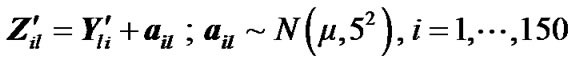
where  is fMRI response or time points matrix of size 150 × 4 and
  is matrix of artificial signals of size

Table 1. Artificial activation in four different regions of interest (ROI).

Figure 3. Three slice views of a volume of fMRI data and the regions inside black circles demonstrated artificial activation areas in the dimension of (xl × yl).
150 × 4 corresponding to the co-ordinates of  four ROIs. The fluctuations of weak and strong artificial signals
  of Gaussian distribution with means μ = (15, 20) and variance
  of four different ROI are also shown in Figure 4.
This 4-D fMRI human brain data consist of 80 volumes or time points or scans and we made this data in the form of alternative blocks of 40 non-active (rest: no artificial signals) and 40 active (task: artificial signals by using model (7) and (8) volumes, beginning with nonactive volumes. 80 acquisitions or volumes were made: 8 blocks and 10 reps in each block for rest and task conditions. In the 10 repetitions block, we assume a task stimulus, and rest conditions for the next 10 repetitions block. Successive blocks alternated between rest and task settled up a blocked paradigm as shown Figure 5, and the design matrix X of size 80 × 2 represented as.
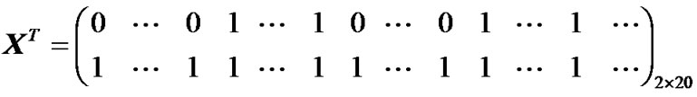
where elements 0’s and 1’s repeated alternatively 10 times in the first row of X for rest and task conditions and all 1’s in second row used only for computation of GLM.
3.2. Analysis of Simulated fMRI Data
The simulated fMRI data were preprocessed and analyzed using SPM latest package (SPM8b; Welcome Department of Cognitive Neurology London) which is based on MATLAB. To avoid the errors, preprocessing steps are necessary before the GLM analysis of any real or simulated fMRI human brain data. Our simulated data
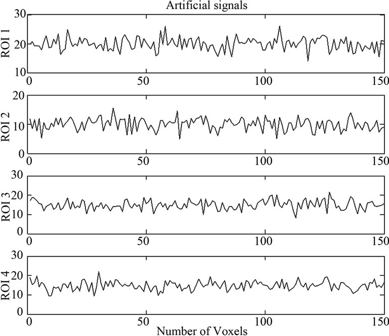
Figure 4. Artificial signals at four ROIs.
Figure 5. Design paradigm of simulation data.
also based on a real fMRI experiment of a subject at resting state. In the preprocessing steps, (1) the whole images data were realigned according to the first volume for the correction of head motion, (2) the images were corrected for difference in slice timing, (3) images were normalized to the Montreal Neurological Institute (MNI) template using parameters defined from the normalization of the anatomical scan to the MNI template and finally, (4) images were smoothed with a Gaussian kernel of 8 mm full-width at half-maximum to reduce noise. For the rest and task conditions of the design matrix X, GLM analysis to estimate  was performed at every voxel of this preprocessed simulated fMRI data by using ReMlL approach of SPM and NH method.
A volume table of SPM {t} maps of the effect β or artificial activity from the whole data were constructed corresponding to the hypothesis “task > rest” at p < 0.001 (uncorrected) level of significance by using the SPM method as shown in Table 2 and by using the NH method as shown in Table 3. A standard volume table of SPM {t} map showed only top three significant voxel of each cluster or region with three digits of p-values and remaining all significant voxels with the full length of p-values (p < 0.001) we showed in the Figure 6. In standard SPM package (SPM8b), any hypothesis must be tested at set-level, cluster-level and voxel-level in the form of adjusted p-values. The columns in volume tables show, from left to right (1) set-level: the chance (p) of finding this (c) or a greater number of clusters in the search

Table 2. Results of the test of simulated fMRI data by using the SPM method where p-values adjusted for search volume in four ROIs.
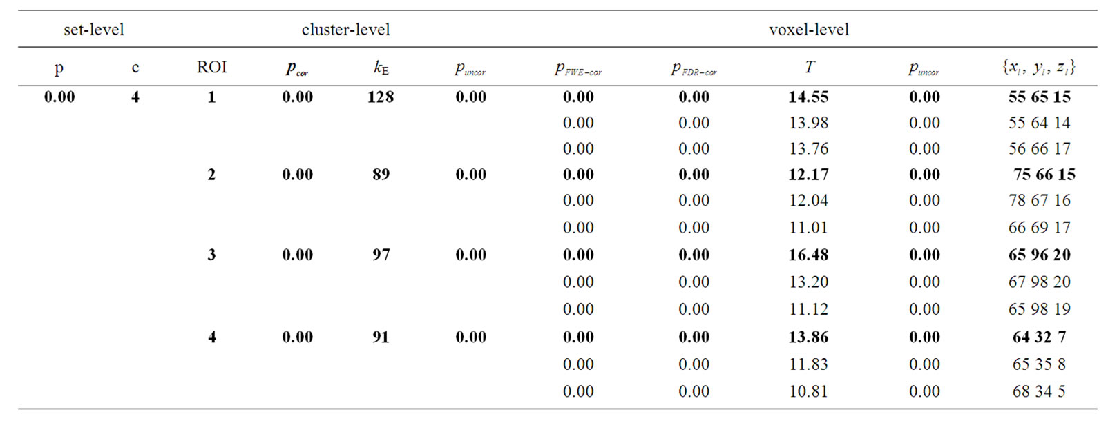
Table 3. Results of the test of simulated fMRI data by using the NH method where p-values adjusted for search volume in four ROIs.

Figure 6. The uncorrected p-values (p < 0.001) of all activated voxels which are tested at voxel-level by using the SPM method (dotted line) and the NH method (solid line).
volume (2) cluster-level: the chance (p) of finding a cluster with this many ( ) or a greater number of voxels, corrected
  and uncorrected
  for search volume (3) voxel-level: the chance (p) of finding (under the null hypothesis) a voxel with this or a greater height (T-statistic), corrected family-wise error
 , corrected false discovery rate
  and uncorrected
 for search volume and (iv),
 : coordinates in the ROIs space instead of MNI space. In the tabular data the bold numbers represents the most “significant” voxel within the cluster at the level p < 0.001 (uncorrected) and there are four significant cluster
  which are our ROI3, ROI1, ROI4 and ROI2 respectively. The number of voxels in the activated ROIs clearly shows that the NH method increases substantially the statistical significance of the four activated regions. Finally, in the analysis of simulated data, the NH method detects, over four ROIs, 20%, 19%, 29% and 27% more activated voxels as shown in Table 3 than the SPM method as shown in Table 2.
A comparison of the two methods is also made with all the uncorrected p-values (p < 0.001) of activated voxel which are tested at voxel-level. The SPM method detected 310 voxels whereas the NH method detected 405 voxels from the total 600 voxels of our four ROIs; the p-values of all the voxels are shown in Figure 6. The figure shows that the NH method has smaller p-values of activated voxels than the SPM. The p-values by the NH method are dispersed over a much wider range than the SPM method which is reflected in the ROC curves described in the Section (3.3) with larger true positive rate and smaller false positive rate for the NH method.
3.3. ROC Curve
We will make use of the well-known receiver operating characteristics (ROC) curve analysis Kim et al. [16] and Fayyaz et al. [15] to compare the SPM and NH methods. A ROC curve is a graphical representation of the true positive rate (TPR) or sensitivity versus the false positive rate (FPR) or (1-specificity) for a binary classifier system over a range of its discrimination threshold. The TPR and FPR values obtained by using the number of true positive (TP) and false positive (FP) activated voxels at specific threshold level in a volume of SPM {t} maps. A volume of SPM {t} maps of both methods corresponding to any p-value or threshold level (T-statistics) can be obtain with the use of SPM package (SPM8b). The TP and FP activated voxels are obtained from the volumes of SPM {t} maps of both methods by applying the lower four sequentially threshold levels as shown in Table 4. Moreover, these obtained TP voxels of simulated data demonstrated those voxels which activated within our predefined areas of ROI whereas FP voxels activated somewhere else in the brain.
In the Table 4, the measures of NH method would yield 496 true positives activated voxels and 1 false positive activated voxel, with a true-positive rate (sensitivity) of 496/599 = 0.8280 and a false-positive rate (1-specificity) of 1/33 = 0.0303. Similarly, 49 true positives and 9 false positives had level between 5.0 and 5.99. Thus, if any value of level greater than 4.99 were taken as an indication of NH method, this measure would yield 496 + 49 = 545 true positives activated voxels and 1 + 4 = 5 false positive activated voxels, with a true-positive rate of 547/599 = 0.9098 and a false-positive rate of 5/33 = 0.1515. And similarly so on for SPM and HM method for the other levels, 4.00 to 4.99, and 3.00 to 3.99.
We plotted true positive verses false positive rates and fitted a simple logarithmic curve (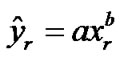 ) to the four bivariate pairs of sensitivity and (1-specificity) for each method, with xr = false-positive rate of activated voxels, yr = true-positive rate of activated voxels. The fitted logarithmic curves represented as the ROC curves of each method as shown below in Figure 7 where solid line curve is for the NH and dots line curve is for the SPM method. The area under the ROC curve from each of the two methods is 95.11% and 89.25% respectively for the NH and the SPM method. The ROC curve and Table 4 demonstrating the superiority of the NH method because
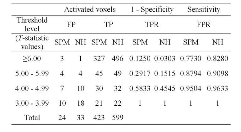
Table 4. ROC curve analysis with the SPM and NH methods.
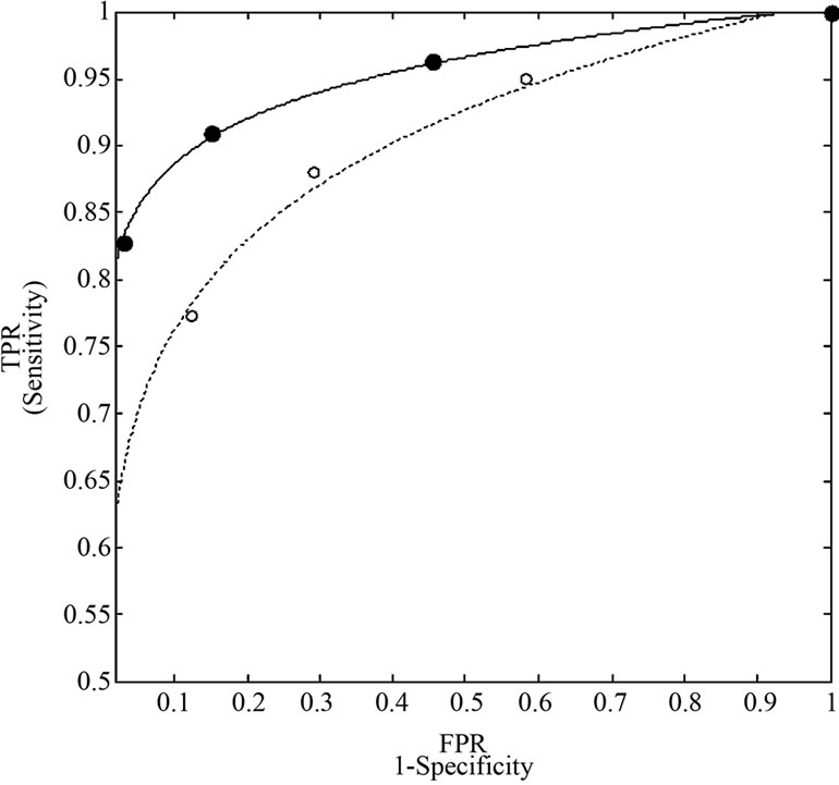
Figure 7. ROC curves for the NH method (solid line) and SPM method (dotted line). The markers represented the points of four bivariate pairs of sensitivity and (1-specificity) of each method.
the NH method has: (1) larger true positive rate; (2) lower false positive rate; (3) larger number of true positive activated voxel; (4) a larger area under the ROC curve by the NH than by the SPM and finally; (5) the closer the curve follows the left-hand border and then the top border of the ROC space, the more accurate the test.
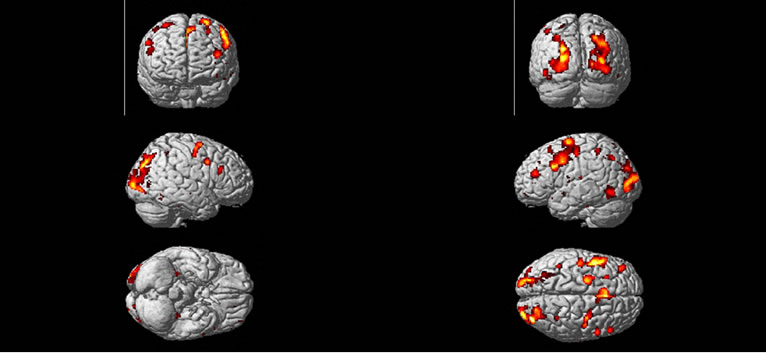
3.4. Real fMRI Data
We also compared the SPM and the NH methods with real fMRI data obtained from a visual block design experiment, which is available in the public domain at http://cnl.web.arizona.edu/spm.htm. The three condition (“study”) block images data were acquired on a GE 1.5T Sigma 5× Wholebody Echospeed Horizon System. The whole brain BOLD/EPI acquisition consisted of 17 slices, each 5 mm thick, with a 1 mm skip (image volume size in voxels: x = 64, y = 64, z = 17 voxel size: 3.44 mm × 3.44 mm × 6 mm; field of view (FOV) is 220). The acquisition took 160 seconds, with the scan-to-scan repetition time (TR) set to 2 secconds. A total of 80 acquisitions were made: 8 blocks of 20 seconds each (i.e., 8 blocks of 10 reps each). During each 20 second block, it was presented 4 stimuli of bird pictures, in each for 5 seconds. Successive blocks alternated between hard and easy learned birds and a control condition of familiar birds (crows and swans), starting with learned birds. The pattern was as in Table 5.
A “2D” T1 anatomical (same plane and section as the BOLD image; Series 2) and a “3D” image (124 Sagittalslices, Series 4) were also acquired to be used as structural images.
3.5. Analysis of Real fMRI Data
We obtained a volume of SPM {t} maps of the condition (“easy and hard > control”) for each method of the above real fMRI data by using the same preprocessing steps (1) to (5) as discussed in the Section (3.2) corresponding to FWE-corrected p < 0.05 and contrast C = [1 –2 1] value. Results are overlaid on a volume rendered brain. The area of activated voxels of each method clearly observed in views of dorsal, lateral and ventral surface of the brain. Yellow and red areas reflect the “easy and hard” condition causing higher brain activities than the control condition as shown in Figure 8. Finally, our proposed method has more activated regions with substantially increased statistical significance, which makes it possible to decide with more confidence if a certain brain region is activated or not.
4. Dicussion
In the NH method, we assume that each voxel is highly spatio-correlated with the neighboring voxels partly due to the smoothing of the data images and we make use of the information from neighboring voxels of a voxel, for estimation at the voxel. Whereas in the SPM, the error covariance matrix, V, does not consider any spatio-correlation among the voxels and hyperparameters of, V, also do not vary over voxels [3,4]. Due this phenomenon some weak signals can not be detected with the use of ReMLE approach of SPM. On the other hand, we admit more heterogeneity of the covariance matrix or variance-covariance structure in the NH method. The distinction of the ROC curves between the NH and the SPM methods becomes more apparent for simulate data as we discussed in the Section (3.3).

Table 5. Block design of a real fMRI data.
 (a)
(a) (b)
(b)
Figure 8. Regions are rendered in yellow and red colors on the MNI template of SPM of activated regions of the brain as a result of “higher active” of easy and hard conditions than the control condition. Active regions detected with the use of the SPM method (a), and the NH method; (b) correspond to p < 0.05 (FWE-corrected).
Worsley et al. [3] used pre-whitening strategy with a spatially varying error covariance matrix V which is repeated at every voxel to estimate regression coefficient β in (2) without using information from neighboring voxels. Zhang et al. [17] and [18,19] used the matrix  to estimate regression coefficient β of whitened model and then applied Durbin-Watson (AR(1) correlation test) on the residuals of whitened model to improve on the accuracy of the autocorrelation model. The variation of the autocorrelation coefficient (ρ) calls for the need for autocorrelation modeling with initial estimates borrowed from neighboring voxels in order to attain more accurate inferences at every voxel.
Finally, In the analysis of simulated data, the NH method detects (405 – 310)/405 = 23% more activated voxels over all the ROIs as shown in Tables 2 and 3 than the SPM method, and real data detects 40% more activated voxels. The proposed method detects voxels more accurately of the simulated data even in case of weak but true artificial signals than the SPM with a better ROC performance. The true positive rate and higher activation of voxels of simulated data showed validity of the proposed method and it is more apparent as far as the real data are concerned. The ROC curves and the p-values of activated voxels show that the NH method is superior than the SPM method based on the true simulated activations.
5. Conclusions
In this paper, we proposed a method in an effort to cope with the heterogeneity of the parameters, in particular the error variance-covariance structure of the noise in the fMRI data. Under the assumption that the parameter estimates do not change abruptly between neighboring voxels, we employed an estimate-transfusion approach between neighboring voxels by using the estimates from neighboring voxels as initial values of the estimates for their new neighboring voxels. Since the intial values may affect the final result of the estimate Wu [20] and Kim [21], it is desirable that we apply the estimate-transfusion approach to obtain the estimates that are affected by the estimates from neighboring voxels.
In both of the experiments, one with artificial data and the other with real data, we showed superiority of the proposed NH method over the traditional SPM method in the context of the ROC curve. In the ReMLE approach of SPM, we assume a variance-covariance structure contains hyperparameters which do not vary over voxels. This may possibly deteriorate the detection accuracy of the activated voxels when the signals are relatively small. This kind of undesirable phenomenon can be avoided by applying the NH method.
6. Acknowledgements
The research reported in this paper has been supported for Sung-Ho Kim through the National Research Foundation of Korea (No. R2011-0026895).
REFERENCES
- C. J. Lueck, S. Zeki, K. J. Friston, M. P. Deiber, P. Cope, V. J. Cunningham, A. A. Lammertsma, C. Kennard and R. S. Frackowiak, “The Colour Centre in the Cerebral Cortex of Man,” Nature, Vol. 340, No. 6232, 1989, pp. 386- 389. doi:10.1038/340386a0
- K. J. Friston, P. J. Jezzard and R. Turner, “Analysis of Functional MRI Time-Series,” Human Brain Mapping, Vol. 1, No. 2, 1994, pp. 153-171. doi:10.1002/hbm.460010207
- K. J. Worsley and K. J. Friston, “Analysis of fMRI TimeSeries Revisited-Again,” NeuroImage, Vol. 2, No. 3, 1995, pp. 173-181. doi:10.1006/nimg.1995.1023
- K. J. Friston, A. P. Holmes, J. B. Poline, P. J. Grasby, S. C. Williams, R. S. Frackowiak and R. Turner, “Analysis of FMRI Time Series Revisited,” NeuroImage, Vol. 2, No. 3, 1995, pp. 45-53. doi:10.1006/nimg.1995.1007
- D. A. Harville, “Bayesian Inference for Variance Components Using Only Error Contrasts,” Biometrika, Vol. 61, No. 2, 1974, pp. 383-385. doi:10.1093/biomet/61.2.383
- P. A. Valdes-Sosa, “Spatio-Temporal Autoregressive Models Defined over Brain Manifolds,” Neuroinformatics, Vol. 2, No. 2, 2004, pp. 239-250. doi:10.1385/NI:2:2:239
- K. J. Worsley, “Non-Stationary FWHM and Its Effect on Statistical Inference for fMRI Data,” NeuroImage, Vol. 15, No. 346, 2002, pp. 779-790.
- P. L. Purdon, V. Solo, R. M. Weissko and E. Brown, “Locally Regularized Spatio-Tem Poral Modeling and Model Comparison for Functional MRI,” NeuroImage, Vol. 14, No. 4, 2001, pp. 912-923. doi:10.1006/nimg.2001.0870
- E. T. Bullmore, S. Rabe-Hesketh, R. G. Morris, C. R. Steven, L. Gregory, J. A. Gray and M. J. Brammer, “Functional Magnetic Resonance Image Analysis of a Large-Scale Neurocognitive Network,” NeuroImage, Vol. 1, No. 4, 1996, pp. 16-33. doi:10.1006/nimg.1996.0026
- N. R. Draper and H. Smith, “Applied Regression Analysis,” 3rd Edition, Wiley Academic Press, New York, 2003.
- B. Everitt and E. Bullmore, “Mixture Model Mapping of Brain Activation in Functional Magnetic Resonance Images,” Human Brain Mapping, Vol. 7, No. 1, 1999, pp. 1- 14. doi:10.1002/(SICI)1097-0193(1999)7:1<1::AID-HBM1>3.0.CO;2-H
- G. S. Watson, “Serial Correlation in Regression Analysis,” Biometrika, Vol. 42, No. 3-4, 1955, pp. 327-341. doi:10.1093/biomet/42.3-4.327
- G. A. F. Seber, “Linear Regression Analysis,” Wiley Press, New York, 1977.
- F. E. Satterthwaite, “An Approximate Distribution of Estimates of Variance Components,” Biometrics, Vol. 2, No. 6, 1946, pp. 110-114. doi:10.2307/3002019
- A. Fayyaz, M. Maqbool and L. Namgill, “Regularization of Voxelwise Autoregressive Model for Analysis of Functional Magnetic Resonance Imaging Data,” Concepts in Magnetic Resonance Part A, Vol. 38, No. 5, 2011, pp. 187-196.
- H. Y. Kim, H. Yong and J. O. Giacomantone, “A New Technique to Obtain Clear Statistical Parametric Map by Applying Anisotropic Diffusion to FMRI,” ICIP, Vol.3, No. 5, 2005, pp. 724-727.
- H. Zhang, W. L. Luo and T. E. Nichols, “Diagnosis of Single-Subject and Group FMRI Data with SPMd,” Human Brain Mapping, Vol. 27, No. 5, 2006, pp. 442-451. doi:10.1002/hbm.20253
- P. A. Bandettini, A. Jesmanowicz, E. C. Wong and J. S. Hyde, “Processing Strategies for Time-Course Data sets in Functional MRI of the Human Brain,” Magnetic Resonance Medicine, Vol. 30, No. 2, 1993, pp. 161-173. doi:10.1002/mrm.1910300204
- S. J. Richard, Frackowiak, K. J. Friston, J. D. Raymond, J. P. Cathy and P. William, “The General Linear Model,” Human Brain Function, 2nd Edition, Willey Academic Press, Oxford, 2003.
- C. F. J. Wu, “On the Converengence Properties of the EM Algorithm,” The Annals of Statistics, Vol. 11, No. 1, 1983, pp. 95-103. doi:10.1214/aos/1176346060
- S. H. Kim, “Calibrated Intials for an EM Applied to Recursive Models of Categorical Variables,” Copmutational Statistical and Data Analysis, Vol. 1, No. 40, 2002, pp. 97-110. doi:10.1016/S0167-9473(01)00 105-0