Open Journal of Radiology
Vol.3 No.1(2013), Article ID:28641,14 pages DOI:10.4236/ojrad.2013.31003
Influence of Tomographic Slice Thickness and Field of View Variation on the Reproduction of Thin Bone Structures for Rapid Prototyping Purposes —An in Vitro Study*
1Department of Pathology, Federal University of Santa Catarina, Florianópolis, Brazil
2Postgraduate Programme on Dento-Maxillo-Facial Radiology, Health Sciences Center, Federal University of Santa Catarina, Florianópolis, Brazil
3Brazilian Institute for Digital Convergence, Federal University of Santa Catarina, Florianópolis, Brazil
4Department of Computer Sciences, Federal University of Uberlândia, Uberlândia, Brazil
5Department of Clinical Medicine, Federal University of Santa Catarina, Florianópolis, Brazil
6Oral and Maxillofacial Surgery, Homero de Miranda Gomes Regional Hospital, São José, Brazil
7Renato Archer Center for Information Technology, Campinas, Brazil
Email: meurer.m.i@ufsc.br
Received July 19, 2012; revised November 30, 2012; accepted December 6, 2012
Keywords: Computed Tomography; Rapid Prototyping; Medical Rapid Prototyping Model
ABSTRACT
This study assessed the influence of acquisition parameters of tomographic volumes on the reproduction of thin bone structures for rapid prototyping purposes. Two parameters were investigated: Field of View (FOV) and Slice Thickness (ST). The specimen was comprised of five pairs of 0.6 mm, 1.1 mm, 1.5 mm, 2.0 mm and 2.8 mm thick cortical bone plates. The plates were stuck into utility wax; the first plate of the pair was in vertical position while the second plate was oblique to the first one. Forty-five tomographic images were captured and separated into 3 groups of fifteen images. Each group had a specific FOV: 180 mm; 250 mm and 430 mm, respectively. Within each of these three groups, tomographic slice thickness was varied for every five of the fifteen slices. Acquisitions were carried out with STs of 1 mm, 2.5 mm and 5 mm. The Cyclops Medical Station software was used in the voxel-to-voxel analysis of radiologic density, reaching a total of 1350 assessed images. ST and FOV variation influenced the reproduction of thin bone walls, and FOV was shown to be a very important parameter. The larger the acquisition FOV, the more reduction in the number of voxels within the range of reconstruction for cortical bone in all of the bone plates. The visual analysis of the images of very thin bone walls showed that there could be a sharp drop in the radiologic density value in several adjacent voxels, resulting in areas which might not be reproduced in the reconstruction.
1. Introduction
The coupled use of CAD (Computer Aided Design) and CAM (Computer-Aided Manufacturing) technologies introduced, in Mechanical Engineering at first, the possibility of creating complex computational models and turn them into solid prototypes through Rapid Prototyping (RP). In the early 90s, this technology was adapted for use in medical specialties [1]. Medical rapid prototyping (MRP) technologies enable the design of physical models of human anatomy and have been used in several specialties, including oral and maxillofacial surgery and dental implantology. MRP models provide important contributions to surgical planning, for example, the intrasurgical decision about the location of osteotomies, reduction in surgical time, increase in surgical safety, reduction in blood loss and specification of shape and contour of prostheses, all of which cause considerable improvement to the treatment’s final outcome [2-9]. Dental implantology has been using these models for surgical planning, especially in more complex cases [10-13]. There are also applications of MRP in tissue engineering and regenerative medicine [14-16].
Attaining MRP models follows a sequence of stages [17]: 1) Acquisition of image data of the anatomy to be modeled; 2) 3D image processing to extract the region of interest from surrounding tissues; 3) Mathematical surface modeling of the anatomic surfaces; 4) data formating for RP and, finally; 5) model design. Despite its reasonable dimensional and geometric accuracy for most clinical applications, three-dimensional reproduction of anatomical data still poses a few problems, and all the steps of the process may be potential sources of errors [3,17,18].
The stage of image data acquisition is extremely important, as the quality of the original data is at the base of the chain that culminates in the production of the MRP model. At this stage, in addition to image acquisition parameters (slice thickness, helical or non-helical acquisition mode, field of view, pitch, gantry tilt, tube current and voltage), reconstruction parameters (including the reconstruction algorithm itself) and patient-related variables (patient movement, metal artifact of intraoral restorations or prostheses) influence the quality of the images acquired.
The stage of image data acquisition is directly related to the next stage: 3D image processing. For the construction of a model that represents only the bone tissue, 3D image processing involves extracting from the dataset the data that correspond to the soft tissue. This process, known as segmentation, is based mainly on the radiologic density of the tissues. In theory, in order to select only bone tissue, it should suffice to delimit the range of radiologic densities which are only bone-related. However, in certain situations, the process of image acquisition does not allow the adequate record of the bone tissue density. Bone tissue might show lower numerical values than those of the typical range for this kind of tissue, which is likely not to be reproduced in the computational model, as a result.
Although computed tomography (CT) is the modality of choice to generate bone MRP models, some authors [3,17-23] have reported difficulty in reproducing thin bone walls (such as anterior wall of maxillary sinus; superior, medial and inferior orbital walls; and small projections, e.g. the anterior nasal spine) and in determining contours to adapt prefabricated prostheses. RP systems enable accurate reproduction of structures that are faith fully represented in the computer-generated model, and this accuracy is subject to variation depending on the technique used; it may be as accurate as 0.015 mm for the stereolithography system. Thus, if thin bone walls are not being reproduced, it may mean that the data related to them were not acquired and/or were omitted from the computational model during segmentation.
The choice for collection acquisition parameters of CT image data drastically interferes with image quality, especially as regards small structures, due to partial volume effect [3,18,19,24]. Given the context above, this study assessed the influence of two parameters which determine the spatial resolution of tomographic data acquisition—1) Field of View (FOV) and 2) Slice Thickness (ST)—on the reproduction of thin bone walls in CTscanned images.
2. Context of the Investigation
For an accurate computational reconstruction of a structure captured in a tomographic volume, the required CT acquisition protocol has to be compatible, at least, with the minimum spatial resolution that can describe all the details of that structure. The determining factor in spatial resolution is the number of space subdivisions, known as voxels, acquired by a CT scanner. The smaller the structure to be captured/represented, the higher the spatial resolution required. When a structure with a very low spatial resolution is acquired, i.e., with voxels of very large dimensions in relation to the size of the structure, parts of the structure may take less than 1 voxel (Figure 1); in this case, the gray level of the image pixel generated for this voxel will correspond to the mean of the radiological densities of all the objects existing in the space volume represented by this particular voxel (the structure, and the air around it, as in Figure 1), resulting in partial volume effect. The partial volume effect corrupts the accuracy of the acquired data as much in contour as in density, which often hinders a three-dimen
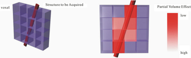
Figure 1. Hypothetical tomographic slice showing a structure acquired with insufficient spatial resolution, with parts of the structure taking space volumes smaller than 1 voxel.
sional reconstruction, or even prevents the accurate geometric measurement of the structure acquired tomographically.
The spatial resolution in the international metric system (SI) can be properly expressed in terms of voxels per cubic centimeter (voxel/cm3) or voxels per cubic millimeter (voxel/mm3). An ideal voxel is a cube of equal x, y and z dimensions (isotropic). Several CT scanners do not enable the capture of tomographic volumes with isotropic voxels, but rather with voxels shaped as cobblestones. This policy has an important consequence when an adequate spatial resolution is sought after for a given structure to be scanned and changes are made to the image data acquisition protocol, because the spatial resolution of a tomographic volume is determined by two parameters which are susceptible to independent adjustment:
• z-resolution: The z dimension of the voxel is given by ST, thus defining a spatial resolution of 1 point per ST, and the amount of voxels in z is given by the number of slices.
• xy-resolution: The number of spatial subdivisions in xy is a constant given by the graphic resolution of the tomographic slice image, typically 512 × 512 pixels in current common tomographs. Consequently, the number of voxels per CT slice is typically constant. The spatial resolution alongside the xy plane can, however, be modified through the change in the size of the space area taken by the square represented by an image of a tomographic slice. This is effected through the change in FOV, which results in an increase or decrease in the side of this square. This way, the x and y dimensions in each voxel are modified, but their amount is not.
Figure 2 shows simplified examples of the influences on spatial resolution caused by changes in the z-resolution and the xy-resolution. Four hypothetical to
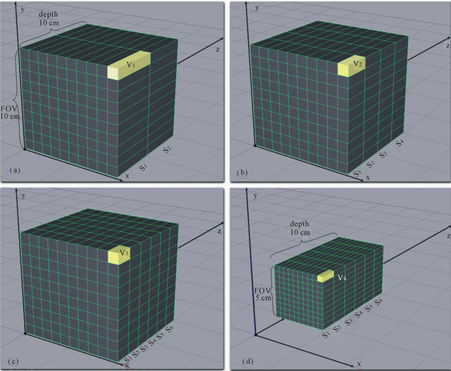
Figure 2. Tomographic volumes with different spatial resolutions showing the influence of the ST and FOV parameters over spatial resolution.
mographic volumes were selected, and they occupied an initial volume of 1000 cm3 (cube with 10-cm side). To simplify the calculation, we assumed that the resolution of the hypothetical tomograph which acquires this volume is 10 × 10 pixels and remains constant. Figure 2(a) shows the acquisition of a tomographic volume of FOV = 10 cm, with two slices S1 and S2 and ST = 5 cm. The dimensions of the resulting voxel v1 are 1 × 1 × 5 cm, and its volume is 5 cm3. Consequently, the spatial resolution of this tomographic volume is 0.2 voxel/cm3. In Figure 2(b), slice thickness was altered and a tomographic volume was acquired of FOV = 10 cm with four slices (S1 to S4) of ST = 2.5 cm. The resulting voxel v2 measures 1 × 1 × 2.5 cm and its volume is 2.5 cm3. Hence, the spatial resolution of this tomographic volume is 0.4 voxel/cm3, i.e., twice as much as the resolution of the previous volume. In Figure 2(c), slice thickness was reduced even further and a tomographic volume of FOV = 10 cm and with six slices (S1 a S6) of ST = 1.67 cm was acquired. The resulting voxel v3 measures 1 × 1 × 1.67 cm, and its volume is 1.67 cm3. Thus, this tomographic volume has a spatial resolution of 0.6 voxel/cm3. Figure 2(d) shows that a different procedure was used and the FOV was reduced, while the same slice thickness from Figure 2(c) was selected, and a tomographic volume of FOV = 5 cm with six slices with ST = 1.67 cm was acquired. The dimensions of the resulting voxel v4 are 0.5 × 0.5 × 1.67 cm, and its volume is 0.41 cm3. In this case, the tomographic volume has a spatial resolution of 2.4 voxel/cm3, four times as much as the spatial resolution of the previous volume, even though the ST was kept constant and the FOV was reduced only by half. This rationale suggests that FOV variation has at least an influence which is equal to (or perhaps greater than) the slice thickness on the spatial resolution of tomographic acquisitions and, consequently, on their accuracy.
2.1. What Resolution Is Required to Attain a Good MRP Model?
When image data are acquired for the design of MRP models, the resolution required is determined by the purpose of designing the MRP model:
• Minimal resolution: for the reconstruction of a structure aimed, for example, only at surgical visualization or application where the accurate reproduction of details or measures is not required.
• Resolution for accurate reconstruction: when the reconstructed object is expected to have accurate measures, enough data must be provided so that the threedimensional reconstruction algorithm that will be used can possibly generate a three-dimensional structure that offers a detailed characterization of the object acquired tomographically.
Three-dimensional digital radiologic objects are formed by voxels that can present connectivity with one another in three different ways (Figure 3), and connectivity is essential in the reproduction of a structure in an MRP model. If an object is edge-connected, as shown in Figure 3(a), it can be reconstructed three-dimensionally, and any of its parts can be measured with a certain degree of accuracy. If parts of an object are only vertexconnected, as in Figure 3(b), it can be reconstructed for the sake of visual representation, but the edge-connected segments cannot be measured because they have null thickness, and as a result, any estimate would be inaccurate. Objects of this class are unlikely to yield an accurate three-dimensional reconstruction. If parts of an object have null connectivity, as shown in Figure 3(c), the object is then divided into disjoint segments, and hence, cannot be accurately reconstructed. Figure 3(b) correlates the concept of connectivity with the required resolution for the design of an MRP model, and represents the minimal resolution for three-dimensional reconstruction. However, in order for objects to have resolution for accurate three-dimensional reconstruction, they must be 100% edge-connected, as in Figure 3(a).
Some reconstruction algorithms use additional tools, and not only consider the radiological densities on segmentation, but also take into account concepts of contour, etc., which can increase their reconstruction capacity.
2.2. What Should Be Considered?
Some authors claim that the definition of the scanning protocol must take into account the purpose—i.e., the production of the MRP model [17,19,25]. Studies reporting the use of MRP models have diverse scanning protocols, based either on the author’s experience or on the protocol previously established for the area and/or for a given CT scanner [18,19,23-26]. ST reduction is seen as the most important controllable parameter at the time of image acquisition to ensure adequate resolution of thin bone structures. Lower ST means greater exposure to radiation, and this should be considered when choosing the most appropriate scanning protocol [19]. The study
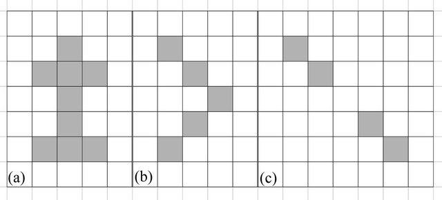
Figure 3. The 3 types of connectivity for two-dimensional representations of objects comprised of quadrangular structures: (a) edge-connectivity; (b) vertex-connectivity and (c) null connectivity.
reported in this article aimed to identify the influence of xy-resolution over spatial resolution and the quality of the data acquired tomographically, through the analysis of the interrelationships among FOV, ST and spatial resolution.
3. Method
The method adopted for this study was divided into 4 steps:
1) Data collection: different combinations of z-resolution and xy-resolution were used in the acquisiton of tomographic images of a specimen, generating datasets with different spatial resolutions.
2) Qualitative data analysis: the acquired tomographic volumes were assessed qualitatively through visual analysis, by means of a radiological workstation tool which provides a voxel-to-voxel data analysis module.
3) Quantitative data analysis: statistical analysis of some of the most remarkable aspects observed, aiming to support the qualitative observation.
3.1. Specimen Design and Image-Data Acquisition
The sample was comprised of 5 pairs of cortical bone plates, taken from a piece of ox bone collected in a meat market. Prior to the plate design, the bone piece was tomographed with 5 mm-thick slices, and the radiological density (in HU) of the cortical bone part was measured.
The bone plates were designed with a Buehler watercooled precision sectioning saw (ISOMET 1000— Buehler, Lake Bluff, EUA), with diamond blades (15 HC DIAMOND, 6" × 0.020"—Buehler, Warehouse, Unionville, Ontario, Canada) and speed range of 600 rpm. Five groups of two plates were then produced, with thicknesses of 0.6 mm; 1.1 mm; 1.5 mm; 2.0 mm and 2.8 mm. The pairs of bone plates were stuck into utility wax. The first plate was placed in vertical position and the second, in oblique position to the first one, yielding an angle of 35 degrees, as shown in Figure 4.
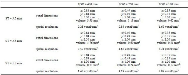
The specimen was placed in the CT scanner (HiSpeed Advantage, GE Healthcare) so that the vertical bone plates were perpendicular to the tomographic slice plane. Forty-five images were taken in non-helical mode, with 120 kVp and 150 mA, which are the bone tissue settings suggested by the manufacturer for this equipment, without slice gap, and with a matrix of 512 × 512 pixels. No image post-processing, filtering or reconstruction methods were applied at the level of the radiological workstation, being all image processing tasks delegated to the data analysis step, described below. Two acquisition parameters were modified when the specimen was scanned: ST (1 mm, 2.5 mm and 5 mm) and FOV (180 mm, 250 mm and 430 mm). As a result, the acquired tomographic volumes yielded 9 different spatial resolutions (Table 1).
3.2. Methodology and Qualitative Data Analysis
The images were analyzed through the use of the Cyclops Medical Station software (www.telemedicina.ufsc.br/ cms/
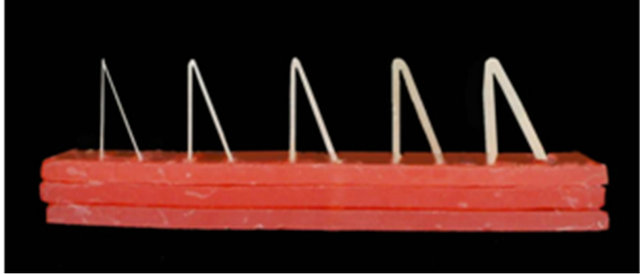
Figure 4. Specimen.
Table 1. Voxel dimensions and spatial resolutions for each of the acquired volumes.
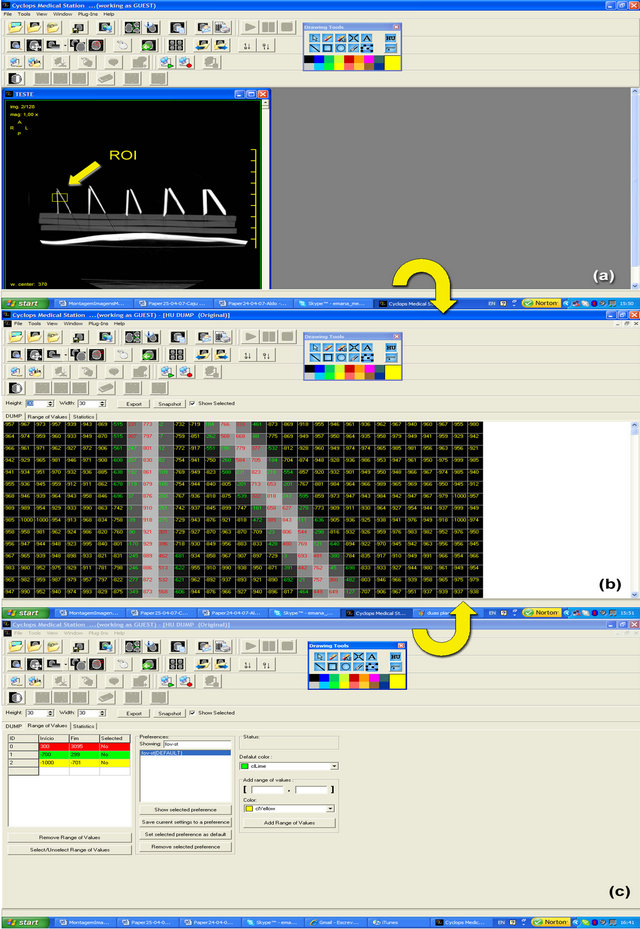
index.php?lang=en), developed by the Laboratory for Image Processing and Graphic Computing (http://www. lapix.ufsc.br) of the Federal University of Santa Catarina (UFSC), in the Cyclops Group (hjttp://cyclops.telemedicina.ufsc.br) and in partnership with the Telemedicine Laboratory (http://www.telemedicina.ufsc.br) of the University Hospital at UFSC. This radiological workstation application offers a model for the analysis of voxel-tovoxel tomographic volumes, which allows for the magnification of image areas and shows each voxel with its radiologic density value in HU. Additionally, this tool enables the delimitation of radiologic density interval ranges, defined by the operator, by coloring the numbers of the varied radiologic density interval ranges in a differentiated fashion (Figure A in the Appendix). For the 3D reconstruction we employed solely the acquired data in the value domain, using the HU values of each voxel accordingly to Wegener [27], considering voxels independently of each other. This was performed without the use of any method in the spatial domain, such as regiongrowing segmentations or morphological kernels, because such methods are based upon general assumptions about data distribution and could introduce false results, e.g. through the closing of gaps in the acquired volume.
Figure A in the Appendix A illustrates the use of this tool in the present study: in figure a region of interest (ROI) in the original image is selected and visualized voxel-to-voxel, together with the respective overlapped HU values. The HU values are displayed in different colors, which represent the different radiologic density interval ranges defined for this study. Voxels in red are located within the tomographic density range defined for the cortical bone (300 to 3095 HU); voxels in yellow are located within the range previously defined as air and noise (−1000 to −701 HU). The definition of the value range for bone tissue was based on Wegener [27], who claims that the HU value range for a compact bone begins at 300 HU in a −1000 to 3095 HU scale. If the images of the specimen were to represent it accurately, they should show voxels in red and in yellow. Nevertheless, one can see a third density range, in green, which corresponds neither to bone tissue nor to air/noise; instead, this range corresponds to partial volume effect (defined, thus, between −700 and 299 HU).
The qualitative analysis was carried out for the five pairs of plates. For each pair, there was the selection of an ROI of approximately 10 × 14 mm, in each of the FOV/ST combinations in Table 1, which yielded a total of 9 FOV/ST combinations × 5 plate thickness = 45 ROIs. These images were analyzed regarding their apparent quality, through the visual comparison of sequences of images with identical FOV and identical ST.
3.3. Methodology for Quantitative Data Analysis
This study was based on the hypothesis that the reduction of spatial resolution both in xy and in z triggers the increase of the partial volume effect. In order to verify whether or not the variation of spatial resolutions in xy and in z affects, in a systematic manner, the quality of the acquired data, the HU density means in the voxels of bone, partial volume and air ranges were calculated, and thus the mean of HU values in each plate was obtained for each acquisition protocol, yielding a total of 1.350 radiologic density means. For the sake of comparison, this study used the tomographic density of 30 random measures involving only the cortical bone in the bone piece tomographed previously to the design of the specimen, whose tomographic density mean was 1572.53 HU. For the purposes of this study, this value was considered the gold standard for cortical bone. Through the analysis of variance (ANOVA), the variation of the radiologic density was compared taking four parameters into consideration: physical thickness of the bone plate, ST, FOV, and plate angle (perpendicular or oblique) in relation to the x axis. These parameters were paired and the data were submitted to several ANOVA analyses in order to assess which factor more markedly influences the partial volume effect expressed as systematic radiologic density loss.
3.4. Methodology for Data Reconstruction and Three-Dimensional Visualization
The 3D reconstruction was carried out through the Cyclops Visualization Toolkit [28,29], another radiological workstation module developed at UFSC. This module implements, with slight improvements, the 3D segmentation and 3D reconstruction methodologies based on the Marching Cubes method [30], the current methodology of choice for radiological workstations; in addition, it uses the Doubly-linked Face Lists (DLFL) methodology [31], also currently considered the state of the art in the field of 3D visualization of radiologic images.
4. Results
4.1. Qualitative Data Analysis
Starting from the set of assessed images, sequences of images were created illustrating the effects of the FOV variation in the reproducibility of bone plates. Figure 5 shows a sequence of images of the 0.6 mm plate acquired with 1 mm ST, with ROIs of identical dimension but with different spatial resolution due to the FOV variation. The images were scaled in order to always show the bone plate with the same apparent size, which enables the size difference for the voxels in each FOV to be viewed.
In the acquisition with FOV = 430 mm, reproduced infailures can be seen in the continuity of the bone struc-
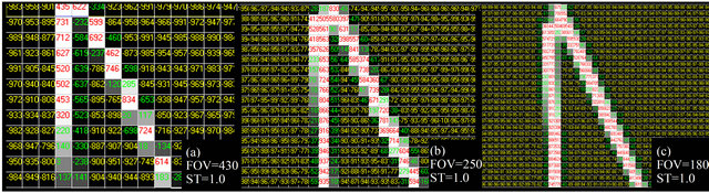
Figure 5. Effect of the FOV variation on the reproduction of bone plates with physical thickness of 0.6 mm, with constant ST of 1 mm. The voxels whose radiologic density corresponds to cortical bone are displayed in red. In the case of a three-dimensional reconstruction, only the voxels in red would be considered. However, their reconstruction in the MRP model would also depend on the connectivity relations among the voxels.
ture, which characterizes null connectivity, as shown in Figure 3(c); this image is not susceptible to 3D reconstruction as a single object. In the acquisition with FOV = 250 mm, reproduced in Figure 5(b), there are no continuity breaks, but only vertex connectivity, as shown in Figure 3(b); this image may be reconstructed three-dimensionally as an only object, but because of its null thickness regions, there may be some accuracy problems in the reconstruction. In Figure 5(c), with FOV = 180 mm, one can note good reproduction of the bone plate, generally with two columns of voxels and edge connectivity along the entire object. This object’s 3D reconstruction is likely to be used for purposes of prototyping considering accurate reconstruction. The apparent quality of the reproduction of bone plates is visibly higher in the FOV of 180 mm; this phenomenon was repeated in a systematic manner for the thicker plates, and the smaller FOV is always the best.
Besides, sequences of images were produced illustrating the effects of ST variation on the reproducibility of bone plates. Figure 6 shows the results for the ST variation in a 0.6 mm plate, with FOV = 180 mm (the best resolution). There is a subtle improvement in the bone reproduction in the image with ST of 1.00 mm; however, it is slight in relation to the apparent quality of the other STs (2.5 mm and 5 mm). The same trend can be seen for the thicker plates, in which the apparent influence of the ST was even smaller, as it was limited to the periphery of the plates.
4.2. Quantitative Data Analysis
The ANOVA analysis using both FOV and ST as category variables showed a significant variation in the tomographic density for all thicknesses of bone plates and of the tomographic slice. The level of significance was 90%. The thicker the bone plate, the greater the tomographic density mean in a same ST. The same occurred for the FOV. It also showed that the tomographic density mean is lower for the plates obliquely positioned in relation to the x axis, when compared to the perpendicular ones. Table 2 has an example of the acquired data; it shows the means for the radiologic densities and for the amount of voxels per density range, ST, FOV and inclination for the 0.6 mm plates, in which the variations are more expressive.
Each line of Table 2 presents the means for the number of voxels and for the values of radiologic density expressed in HU in 5 tomographic slices made with the ST and FOV value shown in the first two columns, yielding a total of 45 tomographic slices per (vertical and oblique) plate. These measures were repeated for the 1.1 mm, 1.5 mm, 2.0 mm and 2.8 mm plates. These data are available for full reference at http://www.lapix.ufsc.br/ST- FOV. For each plate thickness (0.6 mm, 1.1 mm, 1.5 mm, 2.0 mm and 2.8 mm), 8 analyses of variance were carried out, divided into two groups:
- Group 1: Using ST as a categorical variable, with the aim to assess the influence of ST on the partial volume effect:
• 3 ANOVAs describing the radiologic density variation in the bone range in relation to the ST, keeping the FOV constant; an ANOVA for each FOV;
• Radiologic density variation in the bone range in relation to the ST, disregarding the FOV.
- Group 2: Using FOV as a categorical variable, with the aim to assess the influence of FOV on the partial volume effect:
• 3 ANOVAs describing the variation of radiologic density in the bone range in relation to the FOV, keeping the ST constant; an ANOVA for each ST;
• Variation of radiologic density in the bone range in relation to the FOV, disregarding the ST.
The results in each group and the plate thickness were, according to the statistical significance and trend shown, very similar and, for this reason, this section presents, for illustration, only some of the results obtained in the
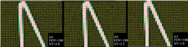
Figure 6. Result of the variation of the ST with a FOV of 180 mm. For this demonstration the 0.6 mm plate was selected, where the acquisition protocol variation produced more expressive changes.
Table 2. Example of the means for the radiologic densities and for the amounts of voxels in each HU unit range, ST, FOV and inclination, showing the results for the 0.6 mm plates.

analysis of the variation of radiologic density in the bone range in relation to the ST and to the FOV for the 0.6 mm and 2.8 mm plates (physical thickness extremes). Figures 7 and 8 illustrate the obtained results. The remaining data are available for reference at http://www.lapix.ufsc.br/STFOV. For the 2.8 mm plate, the same trends were noted, only with much lower significance.
4.2.1. Quantitative Data Analysis in Group 1
Figures 7 (a) and (b) illustrate the results obtained for the 0.6 mm plates. Figure 7(a) shows the results for the analysis of the radiologic density variation in the bone range in relation to the ST for acquisitions with FOV = 180 mm. Figure 7(b) shows the results for the analysis of the radiologic density variation in the bone range in relation to the ST, when performed over all the acquisitions, irrespective of FOV. The trend is slightly more significant with the fixed FOV, but both are very similar.
Figures 7(a) and (b) illustrate the results obtained for the 2.8 mm plates. Figure 7(c) shows the results for FOV = 180 mm and Figure 7(d) shows the results for the independent analysis of FOV. They show the same trend as does the 0.6 mm plate, it only is more evident. In both cases, there is a constant, linear and significant reduction of the radiologic density with the increase of the slice thickness (ST).
4.2.2. Quantitative Data Analysis in Group 2
Figures 8(a) and (b) exemplify the results obtained for the 0.6 mm plates, and Figures 8(c) and (d) exemplify the results for the 2.8 mm plates.
Figure 8(a) shows the results for the radiologic density variation in the bone range in relation to the FOV for the acquisitions with ST = 1.0 mm. Figure 8(b) shows the results for the analysis of radiologic density variation in the bone range in relation to the FOV, when carried out over all the acquisitions, irrespective of ST. The trend is slightly more significant with the fixed ST, but both are very similar.
Figures 8(c) and (d) exemplify the results obtained for the oblique 2.8 mm plates. Figure 8(c) shows the results for ST = 1.0 mm, and Figure 8(d) shows the results for the ST independent analysis, which shows a
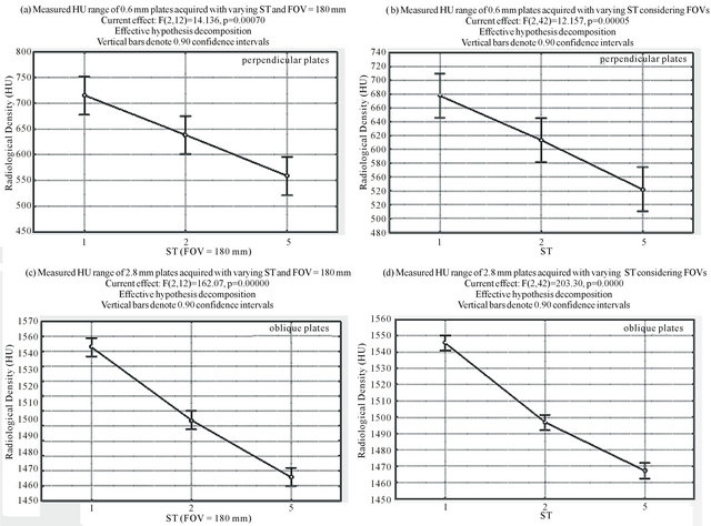
Figure 7. Examples of ANOVA results for Group 1. (a) and (b) display the analyses of perpendicular 0.6 mm plates, and (c) and (d) display the analyses of the oblique 2.8 mm plates.
trend that is very similar to that of the 0.6 mm plate, only it is more evident.
4.3. Three-Dimensional Reconstruction and Visualization of Data
Figure 9 shows the results for the three-dimensional reconstruction of tomographic volumes of the 0.6 mm and 2.8 mm plates, as they represent the extremes of sensibility and robustness of the process. The considerations made in Section 2.1 are confirmed: objects with null connectivity were reconstructed with diverse segments, objects with vertex connectivity show defects that appear as regions without thickness, and objects with edge connectivity are accurately reconstructed. One can also note a slight quality deterioration in the reconstruction of the slices with greater ST, but the determinant factor of quality was the FOV, undoubtedly.
5. Conclusions
The study of the parameters for the acquisition of tomographic images with the purposes of rapid prototyping aims to improve the quality of the MRP model. The dimensional accuracy and the biomodel anatomic details depend mainly on the quality and, consequently, on the spatial resolution of the acquired images, which results from the selection of the scanning parameters and from the CT scanner. Other factors may negatively interfere with the quality of the MRP model (such as the inadequate handling of images), but no later processing can manage to revert the consequences of images acquired under low spatial resolution.
The conclusions drawn from this study are the following:
1) The ST and FOV variations in the protocols for the acquisition of images in this study interfered in different ways with the reproduction of thin bone walls. Nevertheless, they were both shown to have significant influence;
2) The reduction of the spatial resolution, whether through the increase of ST or of the FOV, always led to the reduction in the mean density of the acquired voxels corresponding to bones, which shows direct relation to spatial resolution. An acceptable interpretation is that the variation of both parameters influences the partial vol-
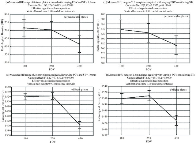
Figure 8. Examples of the ANOVA results in Group 2.
ume effect;
3) The ST variation had much more significant statistical influence on the reduction of the mean of bone than did the FOV variation;
4) The FOV variation had much more significant qualitative influence on the generated images, especially on the quality of the 3D reconstructions, than did the ST variation, which counters the expectations raised by the statistical analysis;
5) In comparison to the tomographic density of the whole piece of cortical bone, thin bone structures (between 0.6 and 2.8 mm) presented lower mean values of tomographic density, and the lower these values the smaller the physical thickness of the bone plate;
6) Bone plates obliquely placed in relation to the axes of the plan of tomographic slice had lower mean values of radiologic density when compared to the values of the perpendicular plates due to greater partial volume effect.
The findings on the influence of the tomographic slice thickness in the reproduction of thin bone plates corroborate reports by Ono et al. (1993), Kragskov et al. (1996), Lightman (1998), Choi et al. (2002), Chang et al. (2003). The increase in the thickness of the tomographic slice was responsible for the reduction of the radiologic density values in cortical bone regions.
On the other hand, this research demonstrated that the FOV variation, as another influence factor on the spatial resolution, also influences the reduction of radiologic density values in thin bone walls. This influence is less statistically significant for the analyzed FOV values, but its consequence for the data qualitative analysis and for the quality of the generated 3D reconstructions is more striking. One possible explanation for this consequence may be the fact that great FOVs drastically reduce the spatial resolution and make the voxels in critical positions of the object be highly influenced by the partial volume effect, which triggers the loss of connectivity and effects such as the occurrence of pseudoforamina and the difficulty in reproducing thin walls such as those of the orbit.
The ANOVA analyses for Groups 1 and 2 show a clear correlation both between the FOV and the radiologic density variation and between the ST and the radiologic density variation. This correlation is more marked and systematic in the relation between the ST and the radiologic density variation, which reflects the
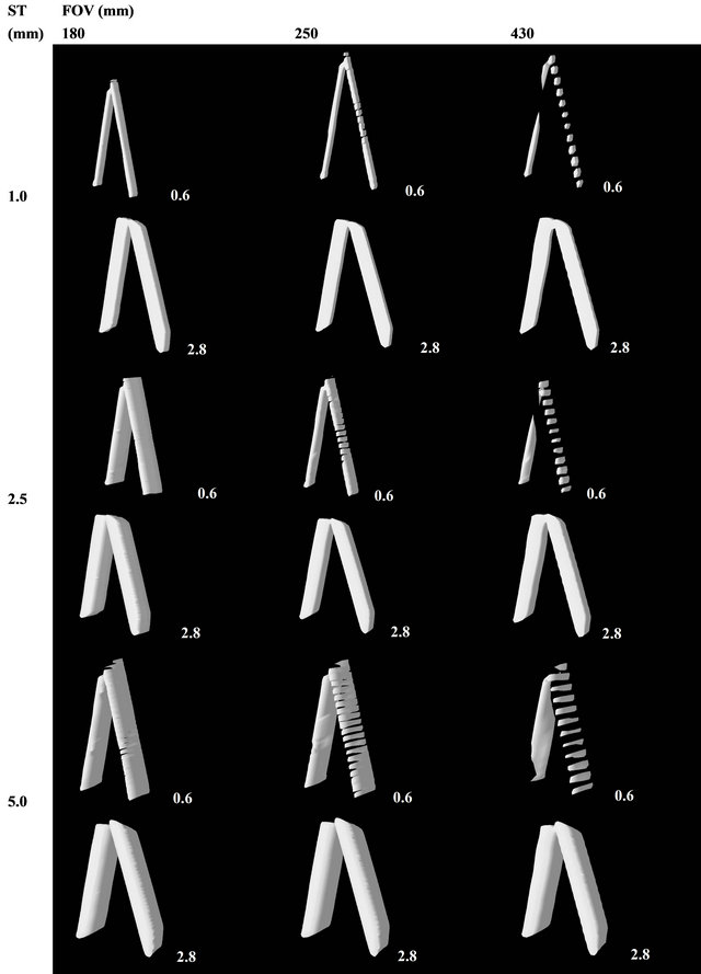
Figure 9. Three-dimensional reconstructions of the 0.6 mm and 2.8 mm plates.
approximately linear relation of 1:2.5 and 1:2 existing between the STs chosen for the experiment. In the case of the relation between the FOV and the radiologic density variation, a marked separation was noted between the 430 mm and the 250 mm FOVs and a much less marked separation between the 180 mm and 250 mm FOVs. This was expected due to the relation 1:1.72 (close to 1:2) existing between the two first FOVs, and the slightly marked relation of only 1:1.39 existing between the 180 mm and 250 mm FOVs.
5. Acknowledgements
The authors would like to thank DMI Clinic—Medical Image Diagnosis, for making their CT scanner available for the acquisition of image data, and the Department of Stomatology at UFSC, for allowing the use of the equipment from the Laboratory of Dental Materials, at UFSC, for the confection of bone plates of the specimen.
REFERENCES
- L. N. J. Mankovich, A. M. Cheeseman and N. G. Stoker, “The Display of Three-Dimensional Anatomy with Stereolithographic Models,” Journal of Digital Imaging, Vol. 3, No. 3, 1990, pp. 200-203. doi:10.1007/BF03167610
- J. Asaumi, N. Kawai, Y. Honda, H. Shigehara, T. Wakasa and K. Kishi, “Comparison of Three-Dimensional Computed Tomography with Rapid Prototype Models in the Management of Coronoid Hyperplasia,” Dentomaxillofacial Radiology, Vol. 30, No. 6, 2001, pp. 330-335. doi:10.1038/sj.dmfr.4600646
- T. M. Barker, W. J. S. Earwaker and D. A. Lisle, “Accuracy of Stereolithographic Models of Human Anatomy,” Australasian Radiology, Vol. 38, No. 2, 1994, pp. 106- 111. doi:10.1111/j.1440-1673.1994.tb00146.x
- P. S. D’Urso, R. L. Atkinson, M. W. Lanigan, W. J. Earwaker, I. J. Bruce, A. Holmes, T. M. Barker, D. J. Effeney and R. G. Thompson, “Stereolithographic (SL) Biomodelling in Craniofacial Surgery,” British Journal of Plastic Surgery, Vol. 51, No. 7, 1998, pp. 522-530. doi:10.1054/bjps.1998.0026
- C. Kermer, A. Lindner, I. Friede, A. Wagner and W. Millesi, “Preoperative Stereolithographic Model Planning for Primary Reconstruction in Craniomaxillofacial Trauma Surgery,” Journal of Cranio-Maxillofacial Surgery, Vol. 26, No. 3, 1998, pp. 136-139. doi:10.1016/S1010-5182(98)80002-4
- G. Santler, H. Kärcher and C. Ruda, “Indications and Limitations of Three-Dimensional Models in Cranio-Maxillofacial Surgery,” Journal of Cranio-Maxillofacial Surgery, Vol. 26, No. 1, 1998, pp. 11-16. doi:10.1016/S1010-5182(98)80029-2
- R. Schön, M. C. Metzger, C. Zizelmann, N. Weyer and R. Schmelzeisen, “Individually Preformed Titanium Mesh Implants for a True-to-Original Repair of Orbital Fractures,” International Journal of Oral and Maxillofacial Surgery, Vol. 35, No. 11, 2006, pp. 990-995. doi:10.1016/j.ijom.2006.06.018
- E. K. Sannomiya, J. V. L. Silva, A. A. Brito, D. M. Saez, F. Angelieri and G. S. Dalben, “Surgical Planning for Resection of an Ameloblastoma and Reconstruction of the Mandible Using a Selective Laser Sintering 3D Biomodel,” Oral Surgery, Oral Medicine, Oral Pathology, Oral Radiology and Endodontics, Vol. 106, No. 1, 2008, pp. e36-e40. doi:10.1016/j.tripleo.2008.01.014
- G. Wang, J. Li, A. Khadka, Y. Hsu, W. Li and J. Hu, “CAD/CAM and Rapid Prototyped Titanium for Reconstruction of Ramus Defect and Condylar Fracture Caused by Mandibular Reduction,” Oral Surgery, Oral Medicine, Oral Pathology, Oral Radiology and Endodontics, Vol. 113, No. 3, 2012, pp. 356-361. doi:10.1016/j.tripleo.2011.03.034
- A. L. Rosenfeld, G. A. Mandelaris and P. B. Tardieu, “Prosthetically Directed Implant Placement Using Computer Software to Ensure Precise Placement and Predictable Prosthetic Outcomes. Part 2: Rapid-Prototype Medical Modeling and Stereolithographic Drilling Guides Requiring Bone Exposure,” The International Journal of Periodontics & Restorative Dentistry, Vol. 26, No. 4, 2006, pp. 347-353.
- K. Lal, G. S. White, D. N. Morea and R. F. Wright, “Use of Stereolithographic Templates for Surgical and Prosthodontic Implant Planning and Placement. Part I. The Concept,” Journal of Prosthodontics, Vol. 15, No. 1, 2006, pp. 51-58. doi:10.1111/j.1532-849X.2006.00069.x
- D. P. Sarment, P. Sukovic and N. Clinthorne, “Accuracy of Implant Placement with a Stereolithographic Surgical Guide,” The International Journal of Oral & Maxillofacial Implants, Vol. 18, No. 4, 2003, pp. 571-577.
- V. N. Viegas, V. Dutra, R. M. Pagnoncelli and M. G. Oliveira, “Transference of Virtual Planning and Planning over Biomedical Prototypes for Dental Implant Placement Using Guided Surgery,” Clinical Oral Implants Research, Vol. 21, No. 3, 2010, pp. 290-295. doi:10.1111/j.1600-0501.2009.01833.x
- N. Sudarmadji, C. K. Chua and K. F. Leong, “The Development of Computer-Aided System for Tissue Scaffolds (CASTS) System for Functionally Graded TissueEngineering Scaffolds,” Methods in Molecular Biology, Vol. 868, 2012, pp. 111-123. doi:10.1007/978-1-61779-764-4_7
- N. E. Fedorovich, J. Alblas, W. E. Hennink, F. C. Oner and W. J. Dhert, “Organ Printing: The Future of Bone Regeneration?” Trends in Biotechnology, Vol. 29, No. 12, 2011, pp. 601-606. doi:10.1016/j.tibtech.2011.07.001
- A. Díaz Lantada and P. Lafont Morgado, “Rapid Prototyping for Biomedical Engineering: Current Capabilities and Challenges,” Annual Review of Biomedical Engineering, Vol. 14, 2012, pp. 73-96. doi:10.1146/annurev-bioeng-071811-150112
- J. Winder and R. Bibb, “Medical Rapid Prototyping Technologies: State of the Art and Current Limitations for Application in Oral and Maxillofacial Surgery,” Journal of Oral and Maxillofacial Surgery, Vol. 63, No. 7, 2005, pp. 1006-1015. doi:10.1016/j.joms.2005.03.016
- J. Y. Choi, J. H. Choi, N. K. Kim, Y. Kim, J. K. Lee, M. K. Kim, J. H. Lee and M. J. Kim, “Analysis of Errors in Medical Rapid Prototyping Models,” International Journal of Oral and Maxillofacial Surgery, Vol. 31, No. 1, 2002, pp. 23-32. doi:10.1054/ijom.2000.0135
- P. S. Chang, T. H. Parker, C. W. Patrick Jr. and M. J. Miller, “The Accuracy of Stereolithography in Planning Craniofacial Bone Replacement,” Journal of Cranio-Maxillofacial Surgery, Vol. 14, No. 2, 2003, pp. 164-170.
- H. Eufinger, M. Wehmoller, A. Harders and L. Heuser, “Prefabricated Prostheses for the Reconstruction of Skull Defects,” International Journal of Oral and Maxillofacial Surgery, Vol. 24, No. 1, 1995, pp. 104-110. doi:10.1016/S0901-5027(05)80870-7
- A. J. Lightman, “Image Realization: Physical Anatomical Models from Scan Data,” Proceedings SPIE, The International Society for Optics and Photonics, Vol. 3335, 1998, pp. 691-694.
- M. C. Metzger, R. Schön, R. Tetzlaf, N. Weyer, A. Rafii, N. C. Gellrich and R. Schmelzeisen, “Topographical CTData Analysis of the Human Orbital Floor,” International Journal of Oral and Maxillofacial Surgery, Vol. 36, No. 1, 2007, pp. 45-53. doi:10.1016/j.ijom.2006.07.013
- I. Ono, H. Gunji, K. Suda and F. Kaneko, “Method for Preparing an Exact-Size Model Using Helical Volume Scan Computed Tomography,” Plastic and Reconstructive Surgery, Vol. 93, No. 7, 1994, pp. 1363-1371. doi:10.1097/00006534-199406000-00005
- J. B. Ahlqvist and A. M. Isberg, “Validity of Computed Tomography in Imaging Thin Walls of the Temporal Bone,” Dentomaxillofacial Radiology, Vol. 28, No. 1, 1999, pp. 13- 19. doi:10.1038/sj.dmfr.4600398
- J. Schneider, R. Decker and W. A. Kalender, “Accuracy in Medical Modeling,” Phidias Newsletter, Vol. 8, 2002, pp. 5-14.
- J. Kragskov, S. Sindet-Pedersen, C. Gyldensted and K. L. Jensen, “A Comparison of Three-Dimensional Computed Tomography Scans and Stereolithographic Models for Evaluation of Craniofacial Anomalies,” Journal of Oral and Maxillofacial Surgery, Vol. 54, No. 4, 1996, pp. 402- 411. doi:10.1016/S0278-2391(96)90109-3
- H. O. Wegener, “Whole Body Computerized Tomography,” 2nd Edition, Wiley-Blackwell, Hoboken, 1992.
- D. Carvalho, T. R. Santos and A. von Wangenheim, “Measuring Arterial Diameters for Surgery Assistance, Patient Customized Endovascular Prosthesis Design and PostSurgery Evaluation,” 19th IEEE International Symposium on Computer-Based Medical Systems, Salt Lake City, 22- 23 June 2006, pp. 225-230.
- B. Tani, T. Nóbrega, T. R. Santos and A. von Wangenheim, “Generic Visualization and Manipulation Framework for Three-Dimensional Medical Environments,” 19th IEEE International Symposium on Computer-Based Medical Systems, Salt Lake City, 22- 23 June 2006, pp. 27-31.
- W. E. Lorensen and H. E. Cline, “Marching Cubes: A High Resolution 3D Surface Construction Algorithm,” Proceedings of the 14th Annual Conference on Computer Graphics and Interactive Techniques, ACM Magazines and Online Publications, New York, 1987, pp. 163-169.
- E. Akleman and J. Chen, “Guaranteeing the 2-Manifold Property for Meshes with Doubly Linked Face List,” International Journal of Shape Modeling, Vol. 5, No. 2, 2000, pp. 149-177.
Appendix A. Brief Illustration of the Process executed to perform the Experiments
The analysis process described in Section 3.2 is illustrated in this Appendix. The images were analyzed through the use of the Cyclops Medical Station software http://www. telemedicina.ufsc.br/cms/index.php?lang=en), developed by the Laboratory for Image Processing and Graphic Computing (http://www.lapix.ufsc.br) of the Federal University of Santa Catarina (UFSC).
This radiological workstation application offers a tool for the analysis of voxel-to-voxel tomographic volumes, which allows for the magnification of image areas and shows each voxel with its radiologic density value in Hounsfield units (HU).
Additionally, the tool enables the operator-defined delimitation of radiologic density interval ranges. This is highlighted in the tool by coloring the numbers of the varied radiologic density interval ranges in a differentiated fashion (Figure A).
NOTES
*Research funded by a grant from FUNPESQUISA—Federal University of Santa Catarina.