Journal of Power and Energy Engineering
Vol.2 No.1(2014), Article ID:42158,10 pages DOI:10.4236/jpee.2014.21003
Nonlinear Control of Interior PMSM Using Control Lyapunov Functions
Department of Electrical and Computer Engineering, Oakland University, Rochester, USA.
Email: msabra@oakland.edu
Copyright © 2014 Maha Sabra. This is an open access article distributed under the Creative Commons Attribution License, which permits unrestricted use, distribution, and reproduction in any medium, provided the original work is properly cited. In accordance of the Creative Commons Attribution License all Copyrights © 2014 are reserved for SCIRP and the owner of the intellectual property Maha Sabra. All Copyright © 2014 are guarded by law and by SCIRP as a guardian.
Received Oct. 31st, 2013; revised Dec. 15th, 2013; accepted Dec. 23rd, 2013
Keywords:Nonlinear Control; Interior Permanent Magnet Motor (IPMSM); Control Lyapunov Function (CLF); IPMSM Experimental Parameter Determination
ABSTRACT
In this paper, we introduce a non-linear torque control for an interior permanent-magnet synchronous motor (IPMSM). The nonlinear control is based on a Control Lyapunov Function (CLF) technique. The proposed stabilizing feedback law for the IPMSM drive is a damping control method and is shown to be globally asymptotically stable. The CLF method takes the system nonlinearities into account in the control system design stage. Such nonlinearities are due to the cross coupling between the q and the q currents in addition to the system parameters like the inductances and the flux linkages. The complete IPMSM drive incorporating the proposed CLF has been successfully simulated in a plant model for both motor and inverter. The performance of the proposed drive is investigated in simulation at different operating conditions. It is found that the proposed control technique provides a good torque control performance for the IPMSM drive ensuring the global stability. In later work, we are planning to investigate other phenomena such as magnetic saturation, nonlinear loads, mechanical friction and flexibilities.
1. Introduction
The permanent-magnet synchronous motor (PMSM) has been gaining popularity especially in the automotive industry mainly due to its relatively high efficiency, small size and robustness. All these advantages result from the high-energy rare-earth alloys. Despite the high cost of these magnets, the PMSM is still the AC drive of choice in the automotive industry. The interior permanent-magnet synchronous motor (IPMSM) referred to as embedded PMSM also has the magnets buried in the rotor core, as opposed to the surface-mount PMSM where the magnets are mounted on the outer surface of the rotor. In addition to a mechanically robust rotor, the IPMSM enables an accurate estimation of the initial rotor position by inductance variations due to motor saliencies.
The advances in both power electronics and control theory had made the high-performance requirements possible by enabling the IPMSM to be operated in highspeed mode in the constant power region. The dynamic behavior of the IPMSM is significantly improved by using vector control theory. The motor variables are transformed from the fixed stator reference frame to the rotor reference frame. Precise control of an IPMSM drive has its challenges due to nonlinear coupling of currents and the rotor speed, as well as the nonlinearity present in the torque equation.
To achieve precise control of PMSM, many nonlinear methods have been studied. The PMSM control proposed in [1] uses the backstepping method which is a nonlinear control method, but the authors assume that id = 0 which cancels many nonlinearities and limits the operating range of the electric machine. Feedback Linearization is also another nonlinear control method used in [2], and the authors are using a surface mount PMSM where Ld = Lq = L, and the torque is a function of iq. But the most widely used technique in industry is a PI controller [3-7]. There are two PI controllers used for the inner loop torque control, one for the d-current and the other for the qcurrent control. Another PI controller is used for the outer speed control loop. The PI controller designs assume that the system is linear below the base speed and add an anti-windup compensation to account for the highly nonlinear behavior in the flux weakening region. Different variations of the anti-windup techniques are presented in [4,5]. Tuning of the PI controller parameters has also proved to be challenging since the same fixed parameters cannot be used across the whole operation range. This resulted in other PI controller designs that were self-tuning as in [6,7]. Those PI controllers have different controller gains in different operating regions. These self-tuning controllers cannot be used in high performance application like the automotive applications with a very wide operating range.
In this paper, CLF method is used as the nonlinear control method that ensures the stability of the system. No decoupling or simplifications are assumed, and the motor parameters are derived experimentally. The method is proven to be versatile in all operating regions, easier to tune, and superior to the response of both the traditionally used PI controllers with anti-windup and the feedback linearization methods.
The paper is arranged as follows: Section 2 describes the nonlinear IPMSM drive model in the dq reference frame. Section 3 describes the experimental method used to obtain the motor parameters using dynamometer measurements, and the nonlinearities are identified and summarized. In Section 4, the theory of Control Lyapunov Function is presented and chosen as the control method. The CLF method proposed effectively compensates for the IPMSM nonlinearities. The results are discussed in Section 5 and finally the conclusion is given in Section 6.
2. Internal Permanent Magnet Synchronous Motor (IPMSM)
The equivalent circuit model of an embedded permanent magnet synchronous machine in the rotor d-q reference frame [8] is shown in Figure 1.
The corresponding mathematical model in (1) shows the direct vd and quadrature vq voltage equations. Note that the motor parameters are not constant but are functions of  and
and .
.
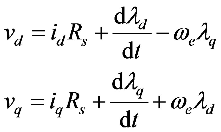 (1)
(1)
where,
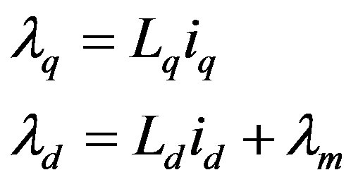 (2)
(2)
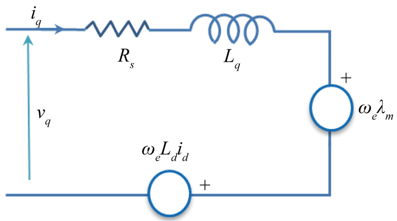 (a)
(a)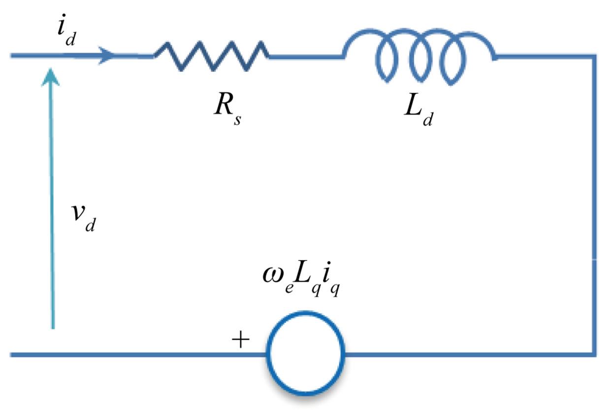 (b)
(b)
Figure 1. Equivalent circuit of an interior PMSM. (a) q-axis circuit; (b) d-axis circuit.
By substituting (2) into (1), we get (3):
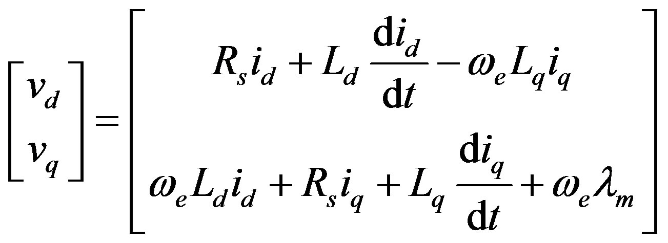 (3)
(3)
The torque equation is shown in (4)
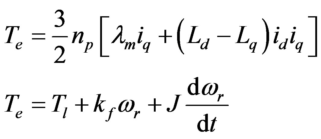 (4)
(4)
where:
 and
and  are the direct and quadrature currents [A]
 and
and  are the direct and quadrature voltages [V]
 is the stator resistance [Ω]
 and
and  are the direct and quadrature inductances [H]
 is the load torque [Nm]
 is the electrical torque [Nm]
 is the moment of inertia of the motor and load
 is the friction coefficient of the motor
 is the rotor angular speed [rad/s]
 is the number of pole pairs of the motor
 is the electric angular speed [rad/s]
 is the permanent magnet flux [Wb]
 and
and  are the quadrature and direct flux linkages
3. Experimental Determination of Motor Parameters
As the speed increases, the nonlinearity of the voltage (3) and torque (4) equations increases. The motor parameters add to the nonlinearity of the system. Therefore, the accuracy of the motor parameters is the first step to improving the control performance of the interior PMSM drives. The parameters are determined to take into account the saturation effects. The effect of temperature however is not taken into account. All measurements are taken at a constant motor coolant temperature.
The IPMSM used is rated at 200 Nm peak torque and 5000 rpm maximum speed with a stator resistance of 10 mohm and 4 pole pairs. The inverter is rated at 100 kW.
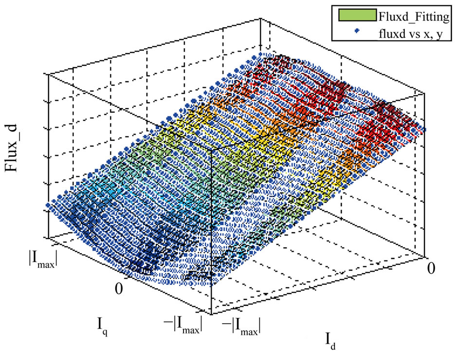
3.1. Flux Linkage λd and λq
To determine λd and λq a test is performed by running the PMSM at constant speed  and sweeping through the motoring and generating quadrants, and by commanding all the possible id and iq combinations. At steady state, (1) becomes
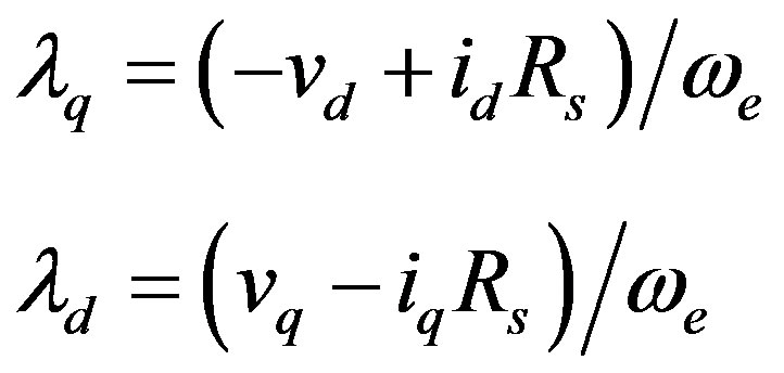 (5)
(5)
By processing the measured phase currents and voltage waveforms, every Id and Iq combination is matched with the corresponding vd and vq. Flux_d  and Flux_q
  are then determined from (5) and shown in Figure 2. The fitting of the flux data as shown also in Figure 2 is used to determine the type of nonlinearity present in the system parameters.
3.2. Permanent Magnet Flux Linkage λm
The permanent magnet flux can be determined by setting the stator currents to zero . Equations (1) and (2) above become:
 (6)
(6)
 (7)
(7)
Therefore,  can be estimated by dividing the fundamental voltage by the electrical angular frequency. Alternatively, to determine
  as a function of
 , the flux
  result has be used. The permanent flux is determined by setting
 . The Permanent flux is therefore
 . The permanent flux is shown as a function of
  in Figure 3.
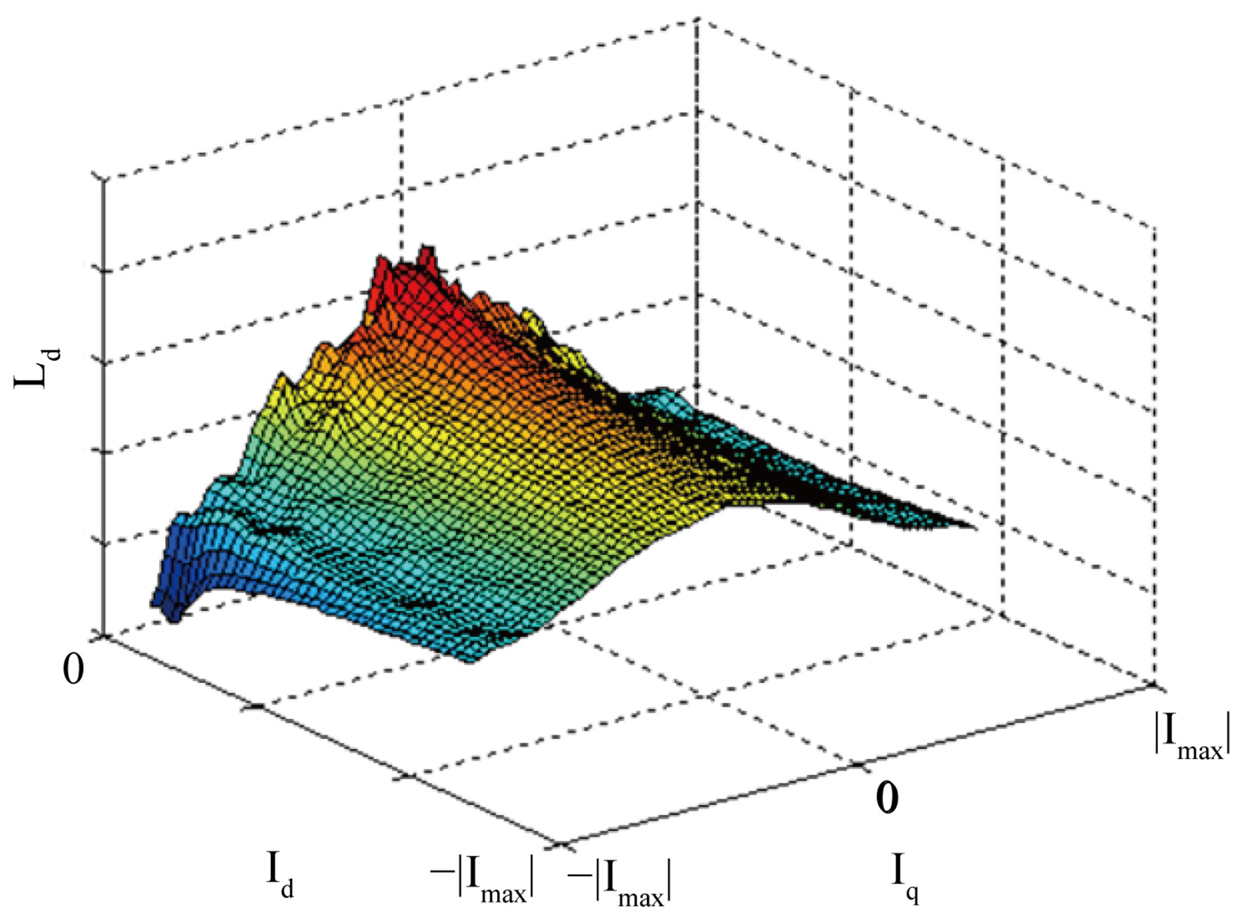
3.3. Inductances Ld and Lq
Ld and Lq are calculated using (2). Ld and Lq are functions of Id and Iq as shown in Figures 4(a) and 4(b) respectivly.
 (a)
(a)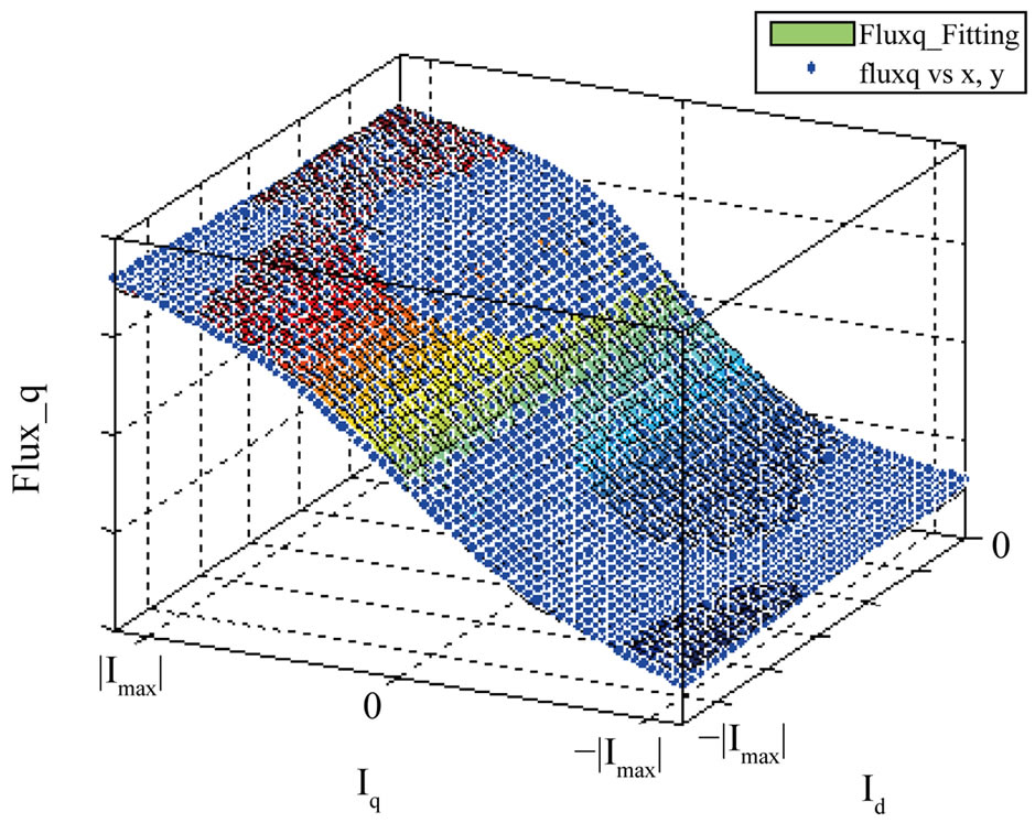 (b)
(b)
Figure 2. (a) Fluxd and (b) Fluxq as a function of Id (x-axis) and Iq (y-axis) (blue: experimental measurements; color map: fitted data). (a) d-axis Flux Linkage; (b) q-axis Flux Linkage.
Figure 3. Permanent magnet flux linkage.
 (a)
(a)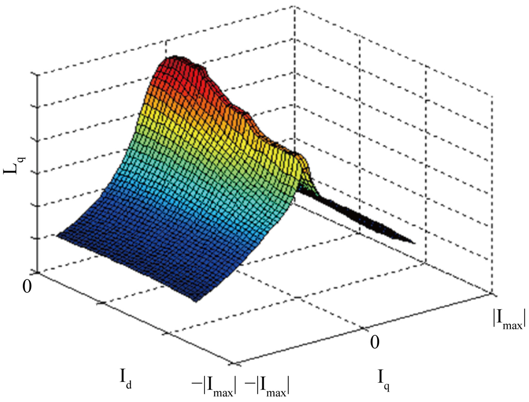 (b)
(b)
Figure 4. (a) Ld and (b) Lq. (a) d-axis Inductance; (b) q-axis inductance.
3.4. Stator Resistance Rs
The stator resistance is determined by measuring the phase-to-phase resistance and calculating the resistance depending on the stator winding having a wye or a delta connection. The stator resistance is a linear function of the stator temperature and will be assumed constant.
3.5. Summary of the Nonlinearities in IPMSM Control
The nonlinearities present in the IPMSM system are due to both nonlinear parameters and the system equations.
The q-axis and d-axis inductances were determined to be function of both Id and Iq and are used as such in the model. But to practical purposes, we can safely assume that Ld and Lq can be fitted into 3 polynomials as functions of Id and Iq respectively without too much impact on the control. The fitting shown in Figure 2 shows that the fluxq and fluxd are sinusoidal functions of Id and Iq. Other nonlinearities are present due to the multiplication of the states as shown in (9) and also in the torque equation The nonlinearities of the IPMSM drive can be summarized in Table 1.
4. Nonlinear Control of IPMSM
The IPMSM drive system used in the simulation is shown in Figure 5. The model consists of the voltage source inverter, the PMSM and two control loops. The inner loop is the current control loop and the outer loop is the speed control loop. Simplified version of this control scheme use the linear decoupled voltage equations for the IPMSM with PI controllers for each of the d and q terms by assuming that the speed and the motor parameters are constant. For speed control an additional PI controller is used for the outer loop control. The motor parameters cannot be assumed constant otherwise the inner loop will be a linear model as in (8).
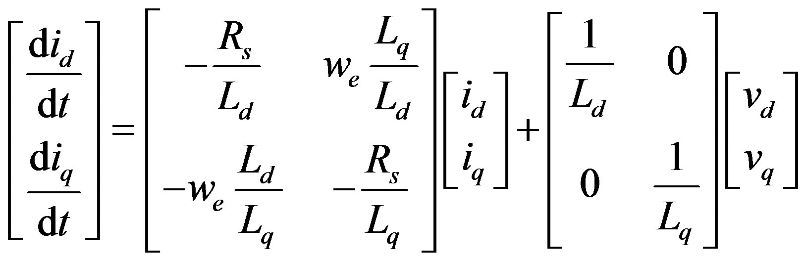 (8)
(8)
This will lead to an unsatisfactory performance of the IPMSM due to the over simplification. This is particularly true during operation in the flux weakening region.
By setting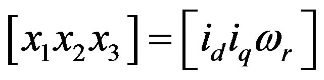 , (3) and (4) can be combined into the nonlinear state Equation (9) to be used
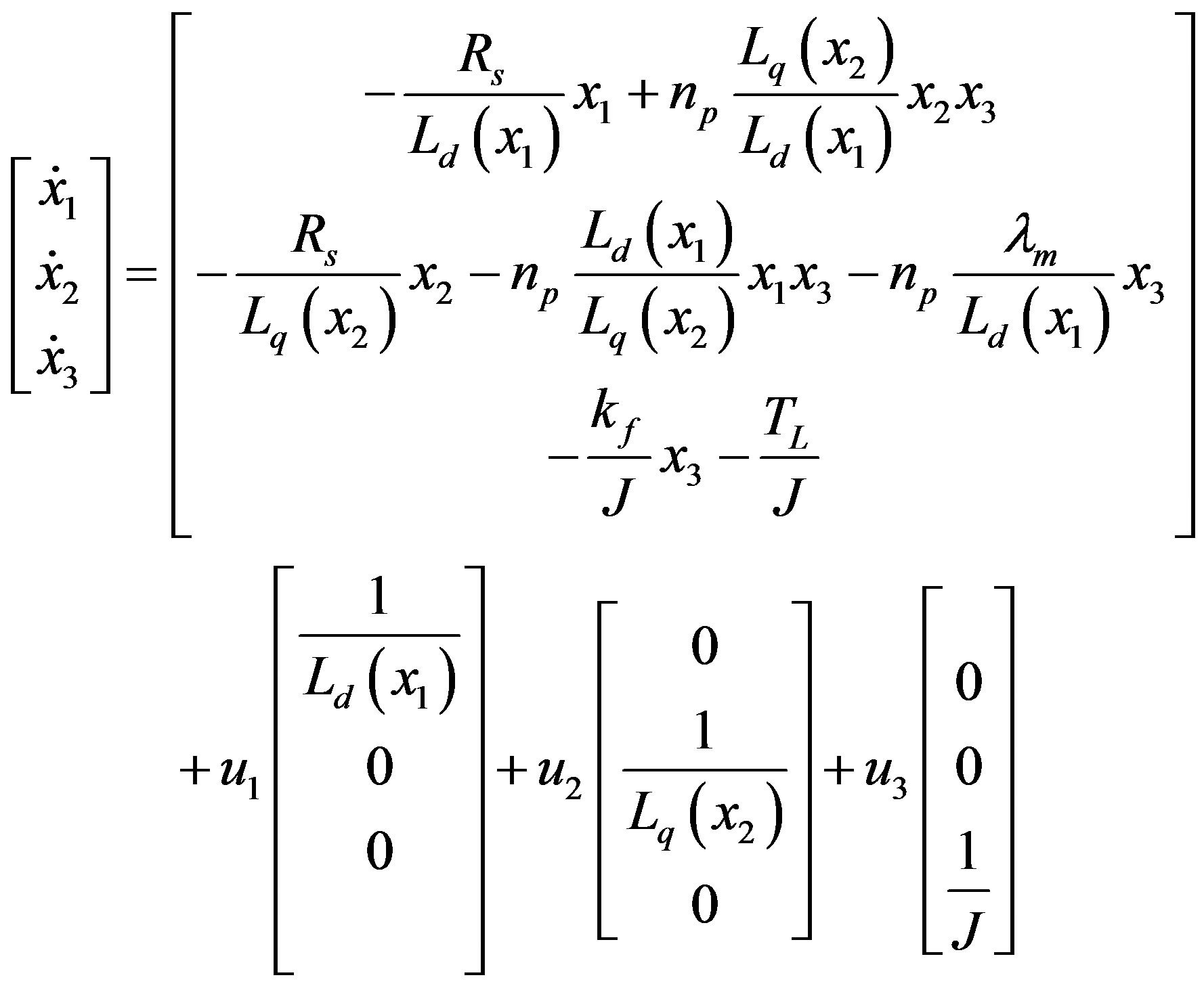 (9)
(9)
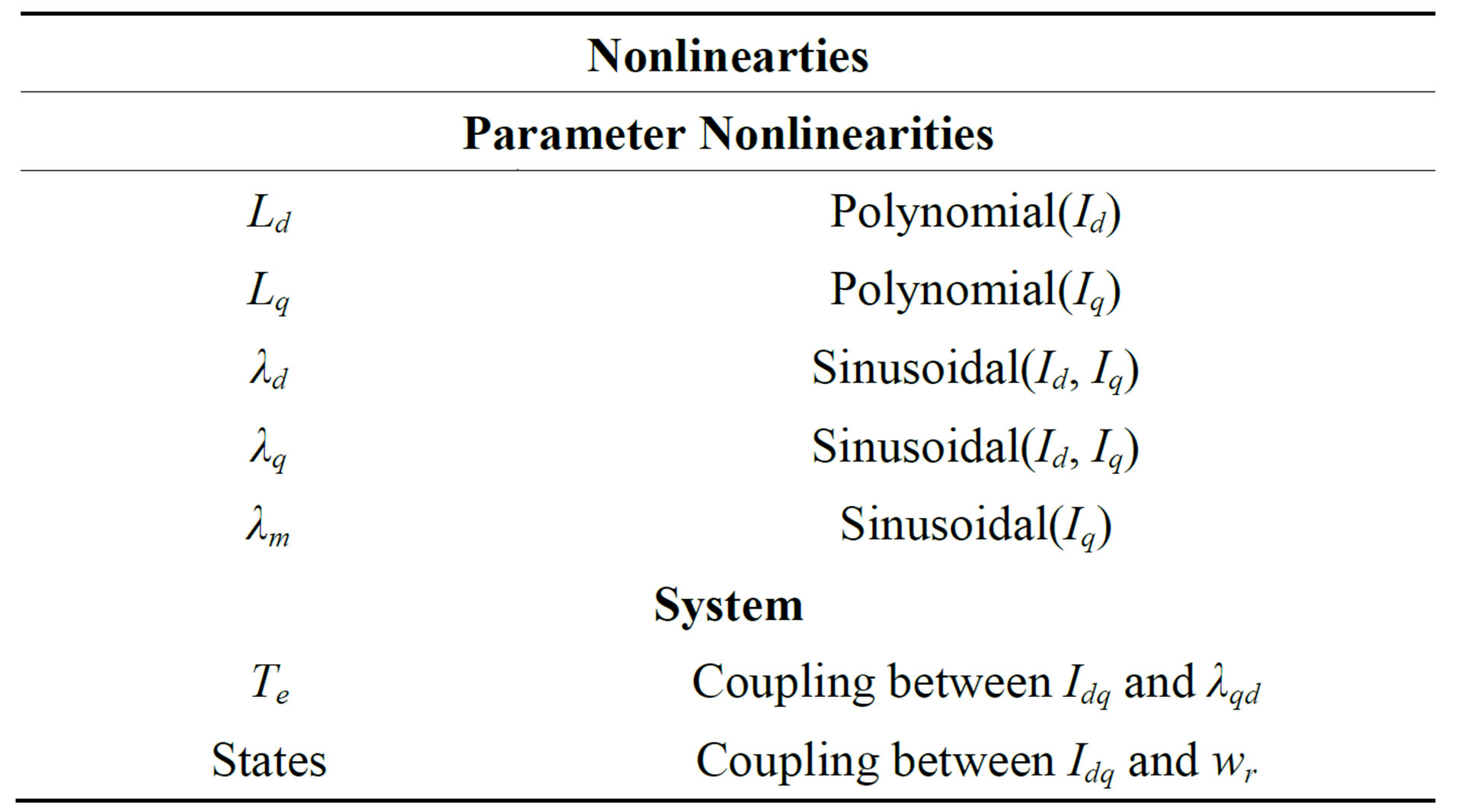
Table 1. Nonlinearities considered in the IPMSM drive.
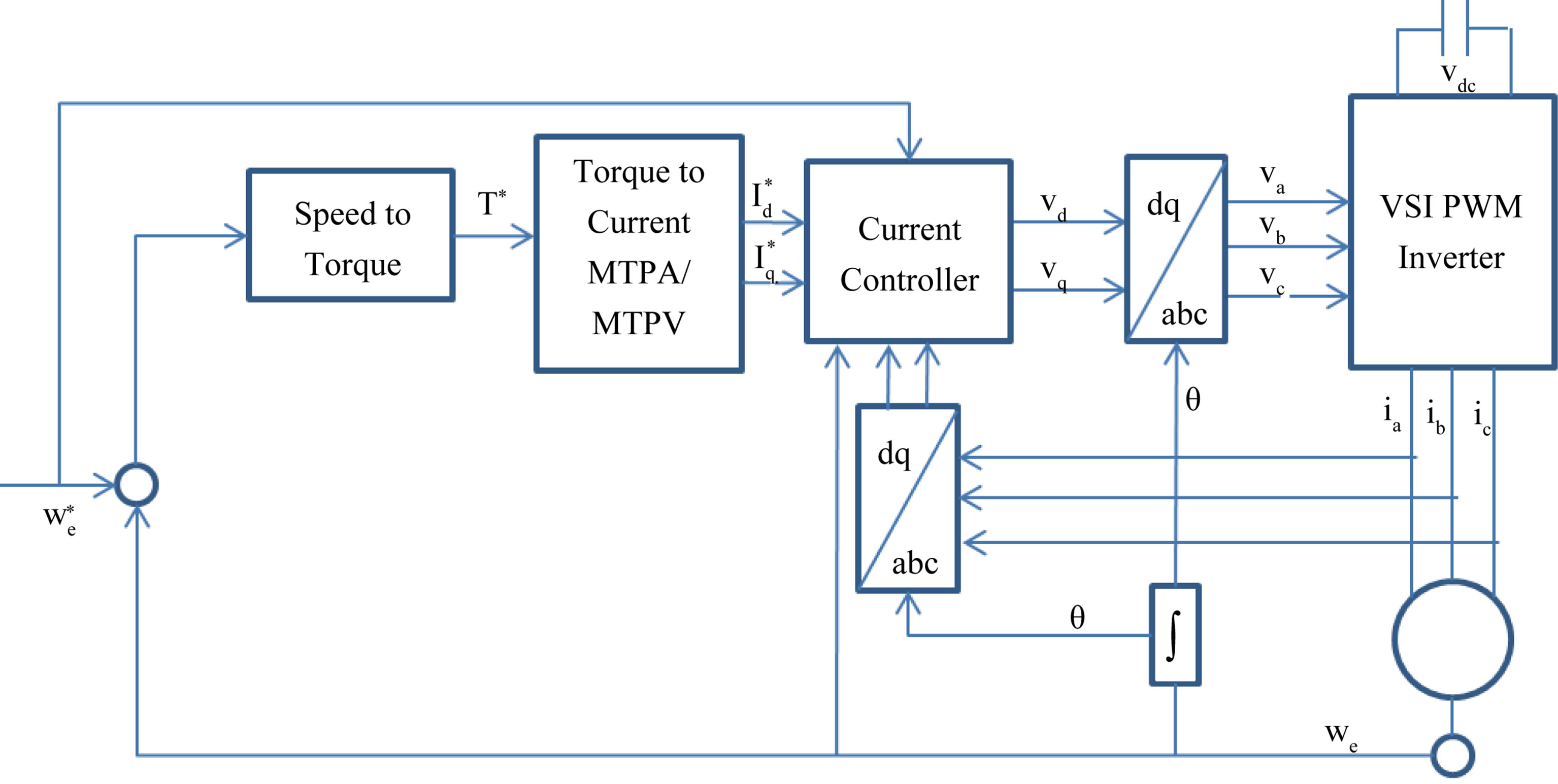
Figure 5. Block diagram of current controlled IPMSM drive system.
where:
(.) operator is the derivative d()/dt x1, x2, and x3 are the systems states u1, u2, and u3 are the control inputs To achieve a high performance control for the IPMSM, Control Lyapunov Function (CLF) method is used. The idea behind this method is to use the system in (9), design a control Lyapunov function, and a control input that minimizes that function. This method does not simplify the nonlinearities that are inherent to the motor model. The proposed CLF method does not assume any simplifications or decoupling in the model. In this section also, a PI control method and a feedback linearization method will be briefly presented to be later compared to the proposed method.
4.1. Control Using CLF
4.1.1. Background on CLF
Consider the non-linear system represented by the state space equation
 (10)
(10)
Where  is the state vector and
  is the control vector. According to [9], the system is said to be affine with respect to the input when it has the form
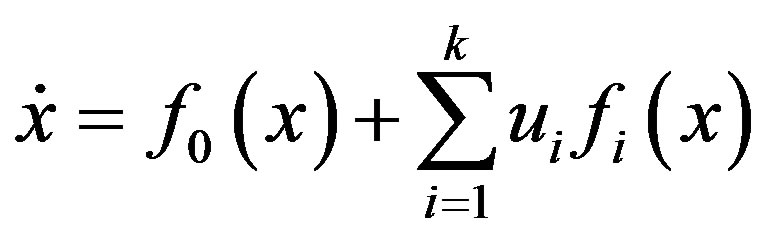 (11)
(11)
where,  are continuous vector fields in Rn.
  is a stable unforced system,
  is the designated control, and
  is a smooth vector field in Rn. When dealing with affine systems, (12) is required.
 (12)
(12)
4.1.2. Choice of a Suitable CLF
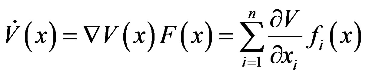
There is no systematic approach for finding Lyapunov functions; in some cases they are natural energy functions for mechanical or electrical systems, in other cases it is just a matter of trial and error [10]. The converse Lyapunov theorems prove that the existence of a Lyapunov function is equivalent to asymptotic stability [11, 12].  is said to be a Lyapunov function of (11) if there exists a region in the neighbourhood of the origin such that:
 (13)
(13)
This region is called the region of attraction [10]
 (14)
(14)
where:
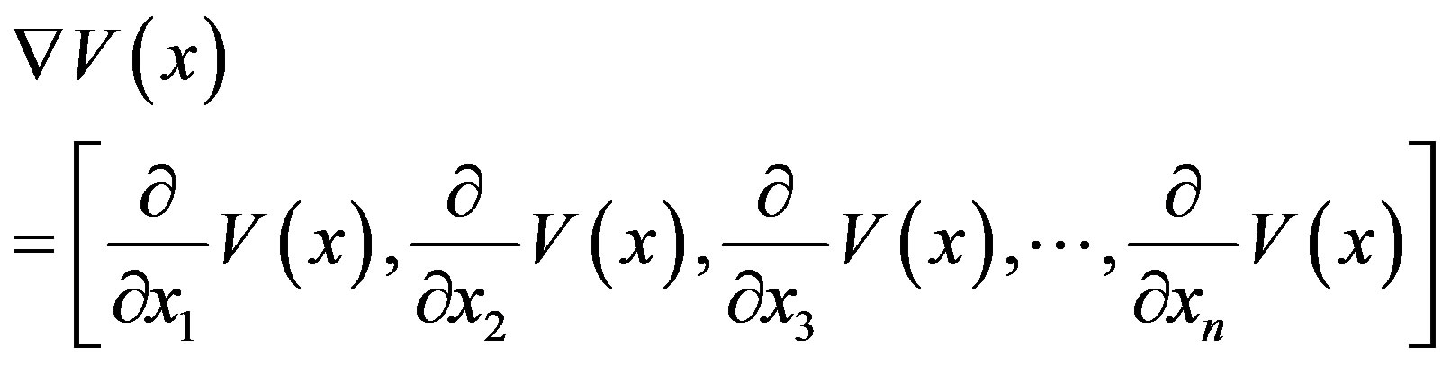 (15)
(15)
The Lyapunov stability theorem states that if (11) has the origin as an equilibrium point and a suitable Lyapunov function V such that ( and
and  for all
 ) and
) and  for all
 , then the origin is stable. In addition if
  for all
 , then the origin is globally asymptotically stable [10]. The selection of CLF is such that V(x) continuously differentiable and positive definite. Stability is guaranteed if
  is positive definite and
  is negative definite for all
4.1.3. The CLF for IPMSM Control
The control objective is torque control. Therefore, the id and iq errors need to be reduced to zero as well as the speed error. Looking at the small scale dynamic model, the load torque term in (9) is canceled.
Different applications have used different types of Lyapunov functions; the authors in [13] have used the natural logarithm and in [14] they used an energy function in their Lyapunov function design. For this application, the selected positive definite control Lyapunov function is defined as in (16)
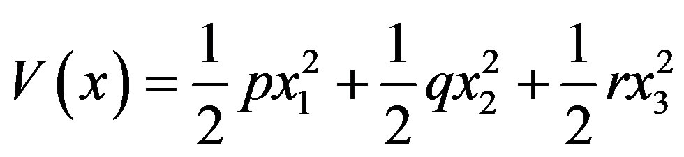 (16)
(16)
where ,
,  , and
, and  are the control parameters
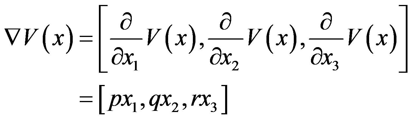 (17)
(17)
The control inputs are chosen as in (18)
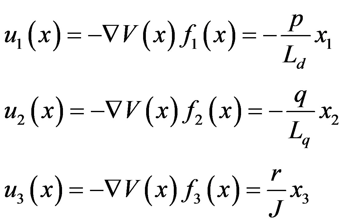 (18)
(18)
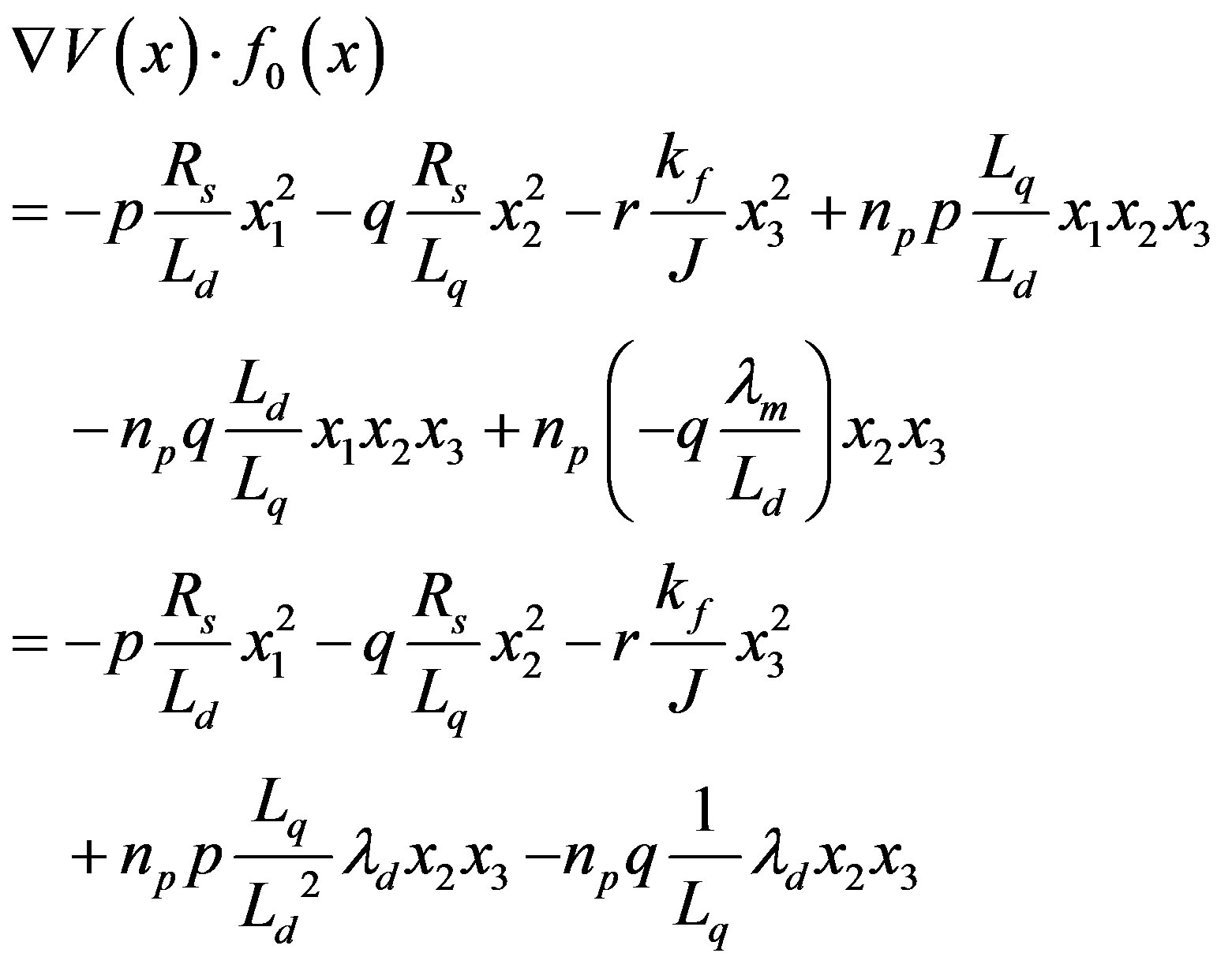
Using the control inputs in (18) and (11), (14) becomes
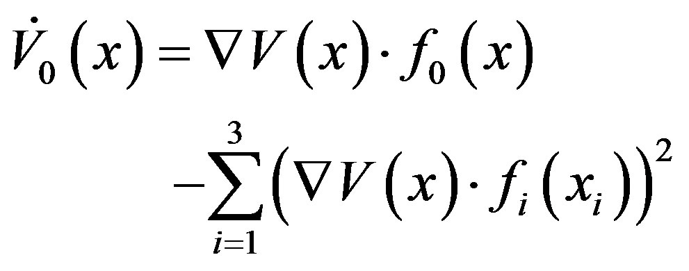 (19)
(19)
For  to be negative definite, the first term
 has to be negative definite.
 (20)
(20)
To ensure the stability of the proposed control, the control parameters are selected as in (21) to guarantee that 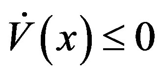 for all x.
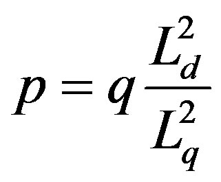 (21)
(21)
The control variables are now reduced to changing one variable as given by (21).
4.2. Control Using a PI with Anti-Windup
The proportional-integral (PI) controller is still widely used in the control of PMSM. However; to account for the nonlinearities due to magnetic saturation, different anti-windup strategies for the integral term have been used. The authors in [4] compare the performance of four different anti-windup designs: Dead zone, tracking, tracking with gain, and conditioned.
For comparison purposes, a PI controller with conditioned anti-windup is used. Figure 6 shows the block diagram of the PI controller used where the integrator holds its last value by setting the output of the anti-windup block to zero when the saturation flag goes high. The parameters used for the PI controllers are Kp = 3 and Ki = 0.01.
4.3. Control Using Feedback Linearization
The main idea of the feedback linearization control is to transform nonlinear system dynamics into linear dynamics by canceling the nonlinearities. As in [2], exact feedback linearization is applied to the inner loop by utilizing the auxiliary inputs in (22). For comparison purposes, feedback linearization is also implemented and its performance is compared to the proposed CLF method.
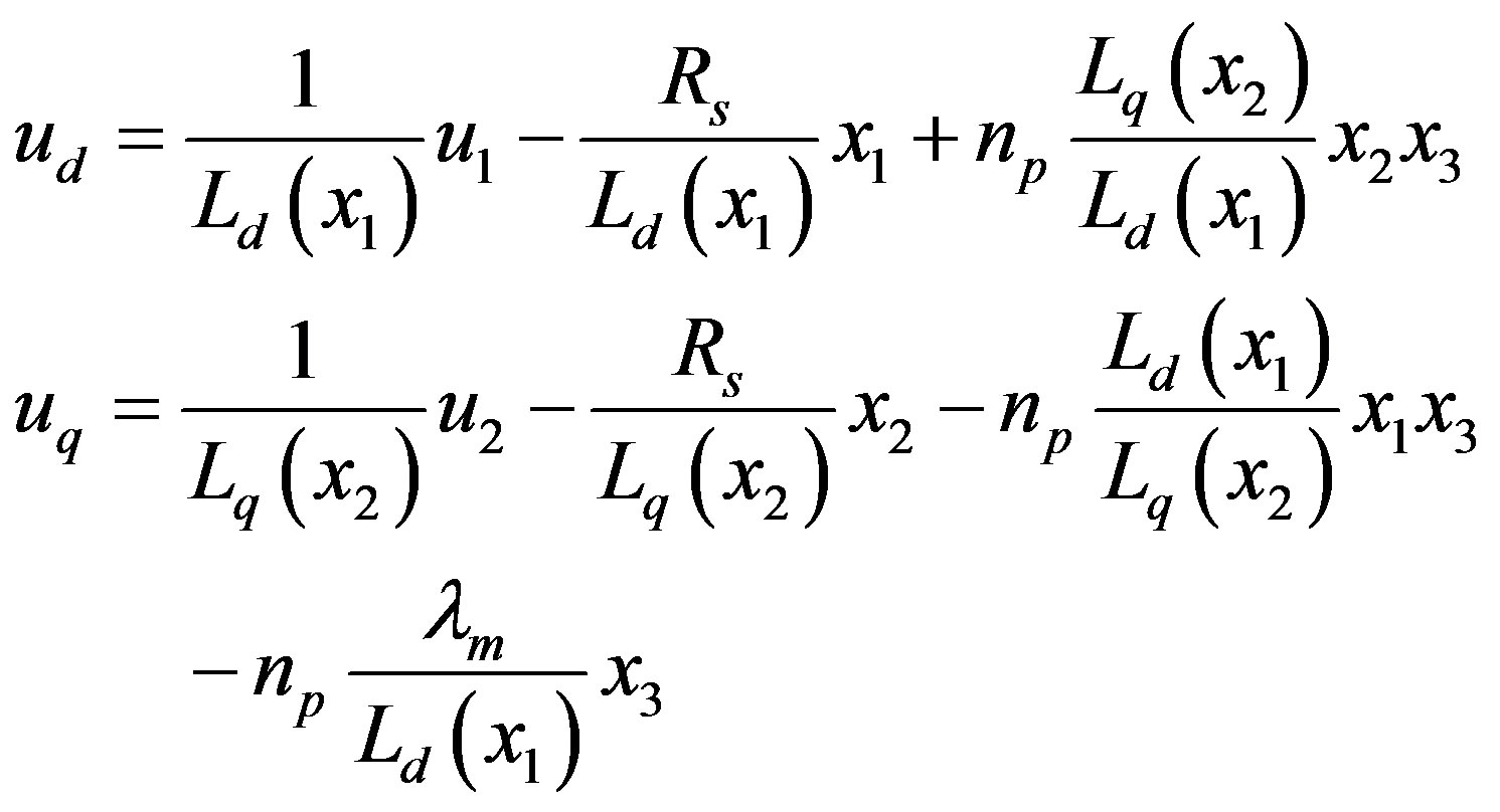 (22)
(22)
5. Results
For a fixed torque command, many current vectors can be commanded. For optimal current vector determination, the operation of inverter fed PMSM drives can be categorized into 2 modes: The constant torque mode which is below the base speed and the constant power mode which is above the base speed. The base speed varies with voltage.
The constant torque operation is shown in Figure 7(a) as Region I. This mode of operation is along the maximum torque per current (MTPC), also known as maximum torque per amperes or MTPA.
As the speed increases from base to maximum speed, the PMSM enters the constant power mode shown in Figure 7(b) as Region II and III. This is also known as the constant voltage mode. The high speed constant vol-
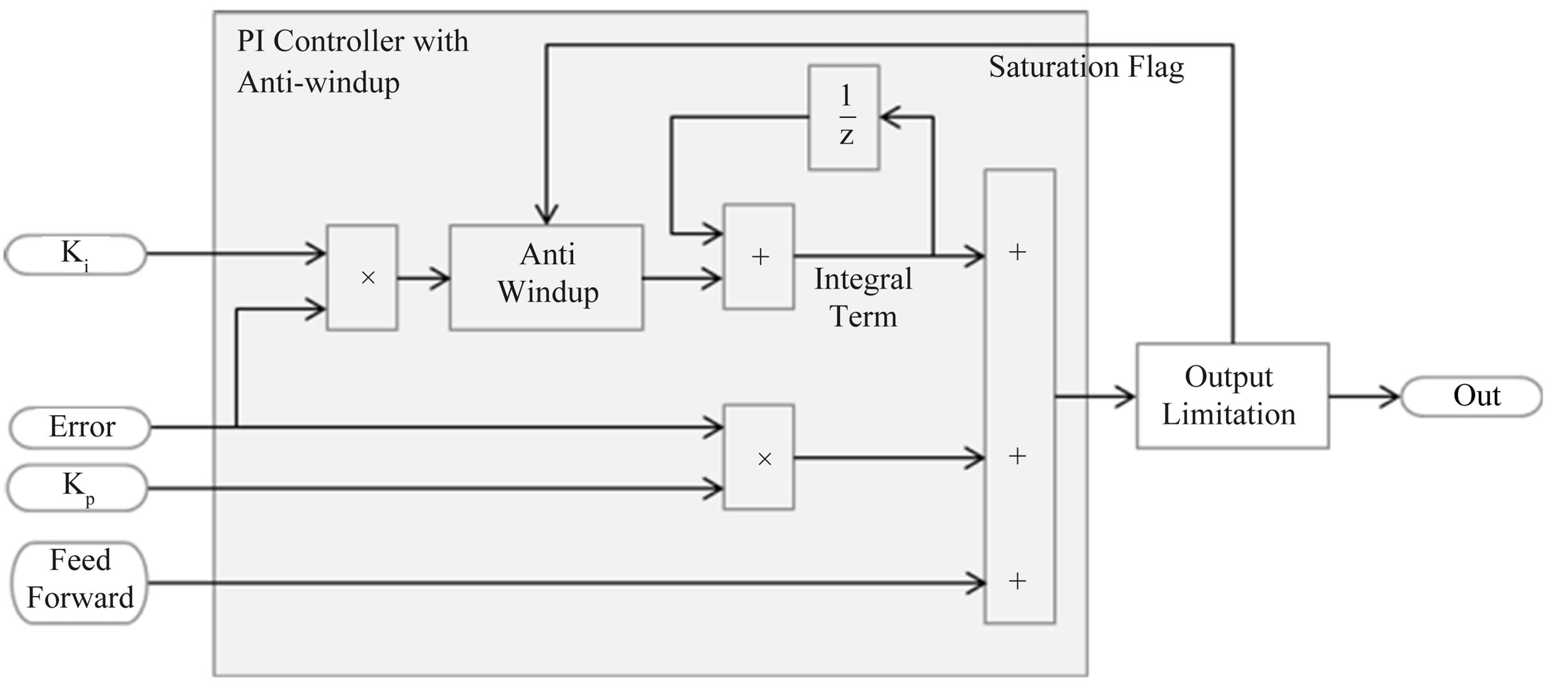
Figure 6. PI controller with anti-windup.
 (a)
(a)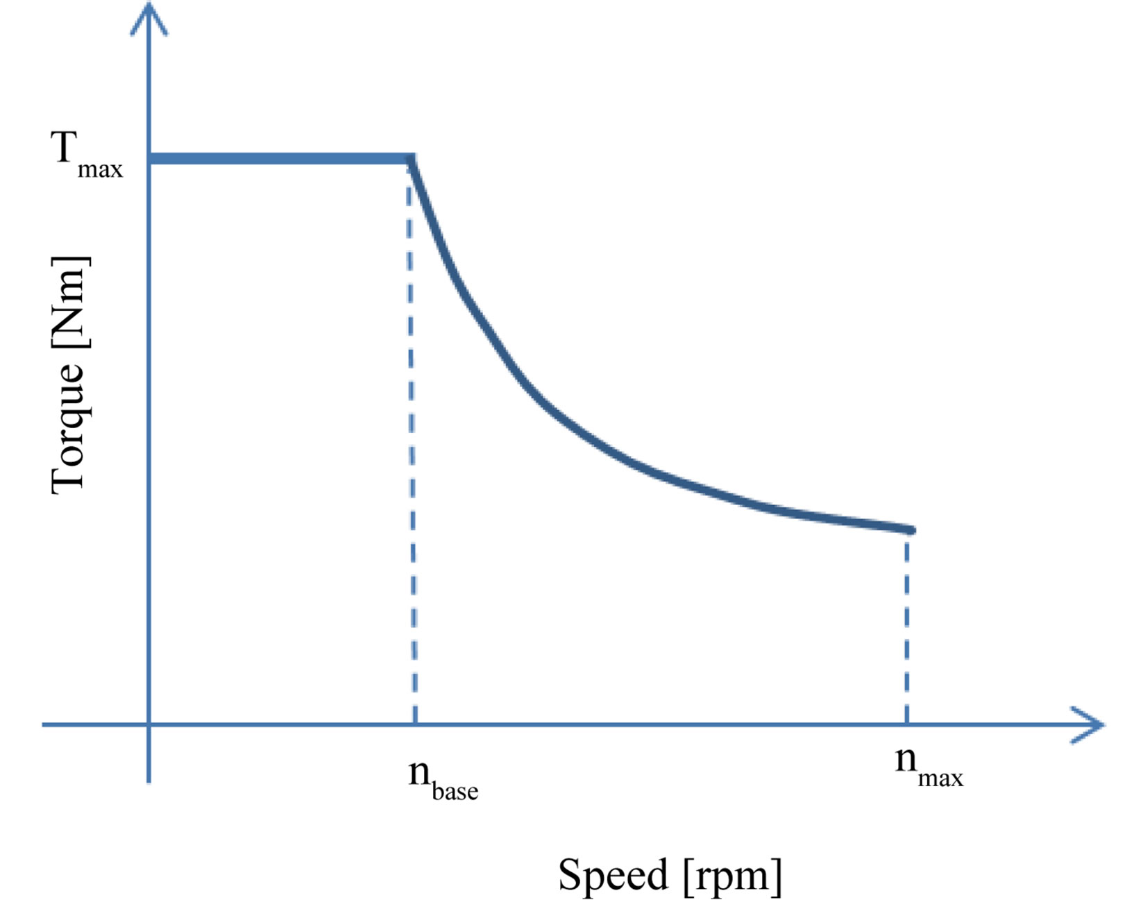 (b)
(b)
Figure 7. Operation regions of IPMSM drive. (a) In the id/iq plane; (b) In the torque-speed plane.
tage operation is realized by reducing the stator flux linkage. Region II and III therefore represent the fluxweakening operation. Region II represents the current limit due to the inverter hardware limitations. Region III is given by the voltage-limit ellipse in the Id-Iq plane as shown by the dashed lines in Figure 7(a). The voltagelimit ellipse becomes smaller as the speed increases and, as a result, the current vector producing maximum torque cannot satisfy the voltage constraint above the base speed.
In this paper, the optimal flux control will be used to achieve the highest PMSM efficiency and wider operating range. In [1], by setting id = 0, the authors designed their control method with a current vector equal to iq. which is more applicable to surface mount PMSM but not very practical for IPMSM.
The performance of the proposed method is verified in this section and compared to the response of both the PI controller and the feedback linearization.
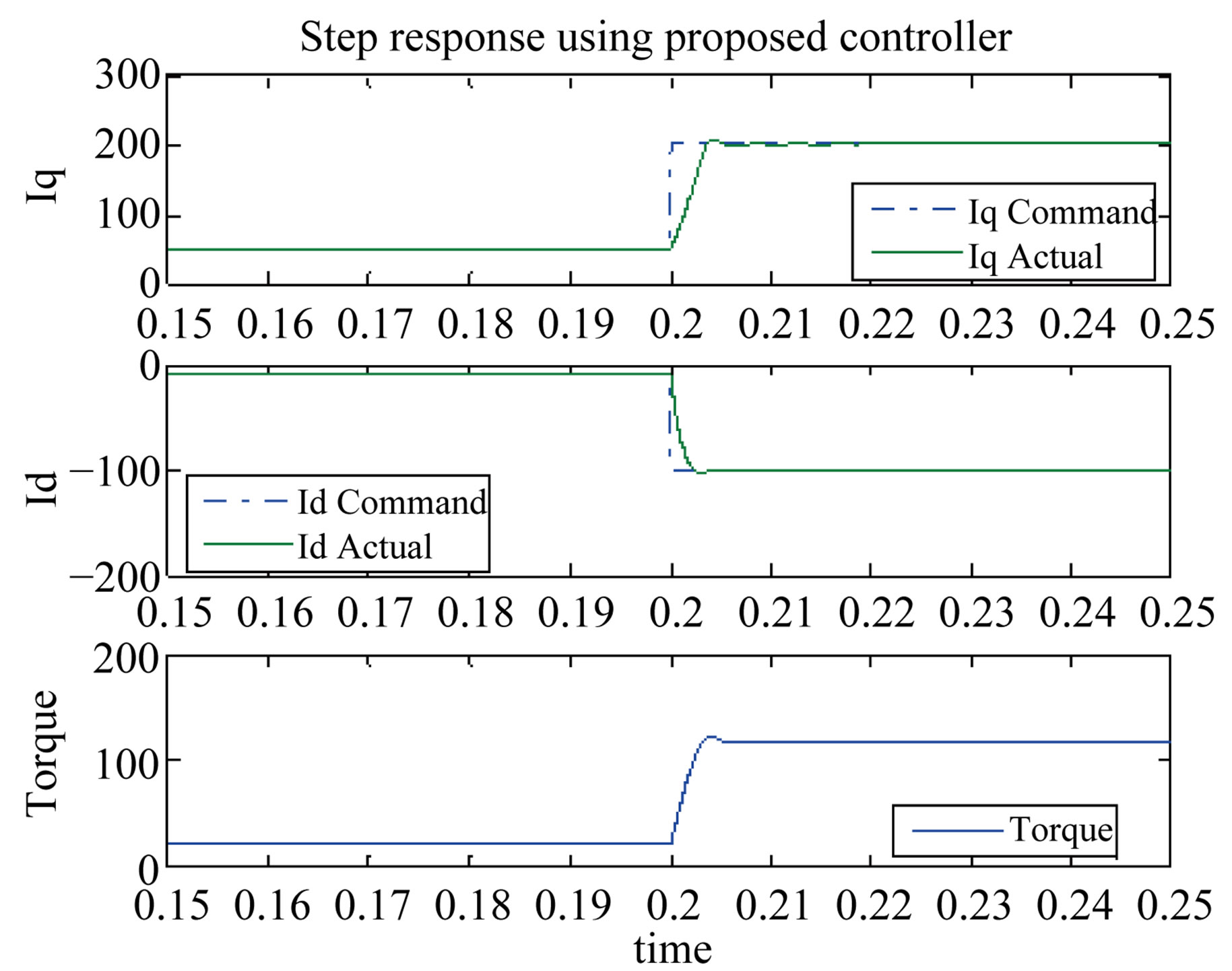
Compared to both the PI control with anti-windup and the feedback linearization, the proposed CLF method shows a very stable response in all regions of operation with no oscillations or overshoots.
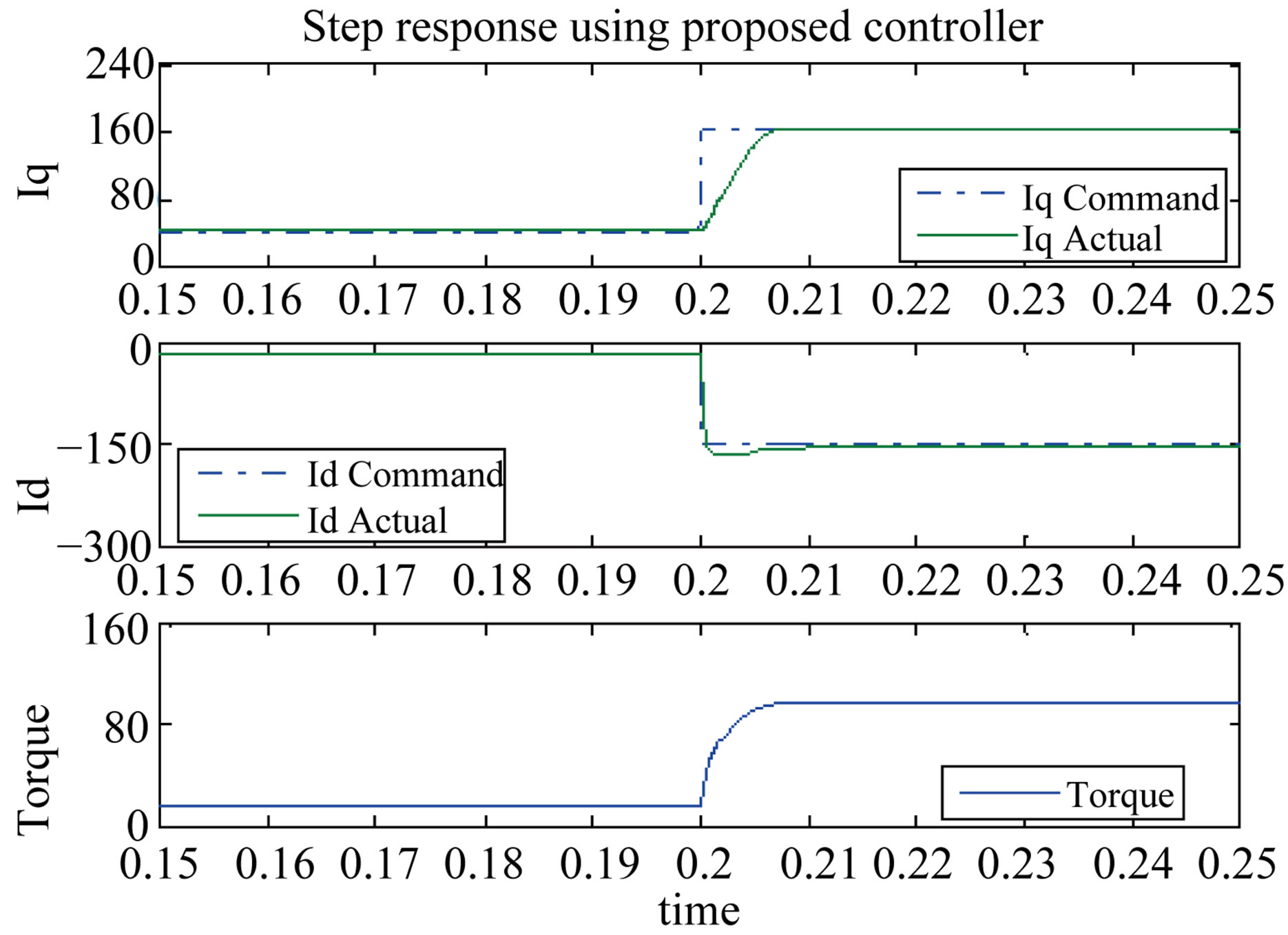
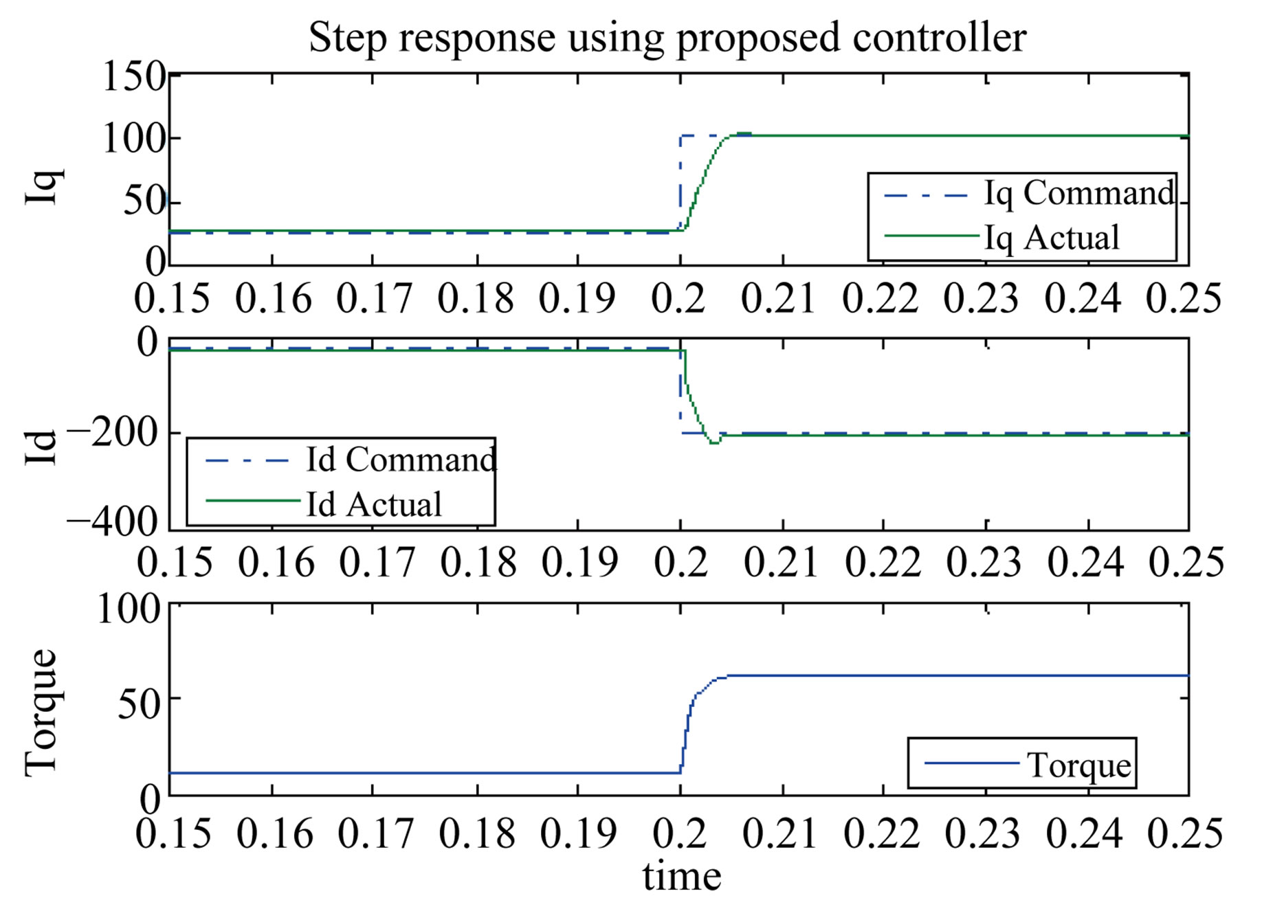
Figures 8-10 each shows a step in torque in Region I, Region II, and Region III respectively where the commanded and the actual current and torque are shown.
The step response using the CLF approach is compared to that of a PI controller with anti-windup and the feedback linearization method. The response of the CLF is superior to those of the feedback linearization and PI controller. Using the CLF approach resulted in less overshoots and no oscillations. The feedback linearization method has lower overshoot in Region I but worse response in Region II and Region III at higher speeds.
The CLF method was easy to tune since only one control parameter needed to be changed. Tuning the feedback linearization method is not straightforward since the response got worse with speed no matter how fast or slow the tuning is. Each PI controller has two gains to be tuned. Tuning the two coupled PI controllers is very difficult especially at high speed and is a topic for a
 (a)
(a) (b)
(b)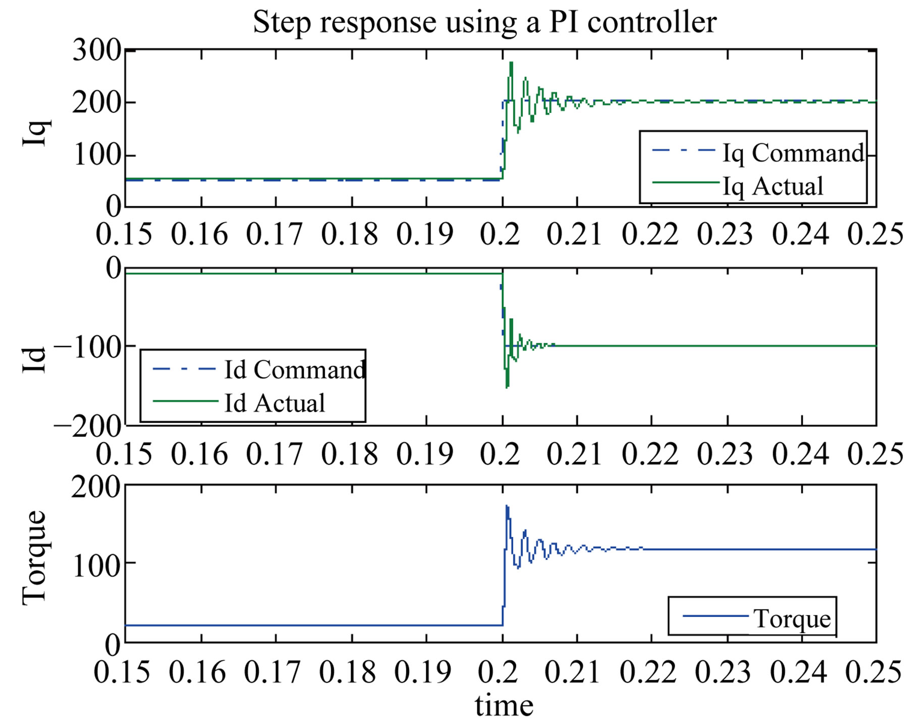 (c)
(c)
Figure 8. Torque and current response (500 rpm). (a) CLF; (b) Feedback linearization; (c) PI controller.
different study.
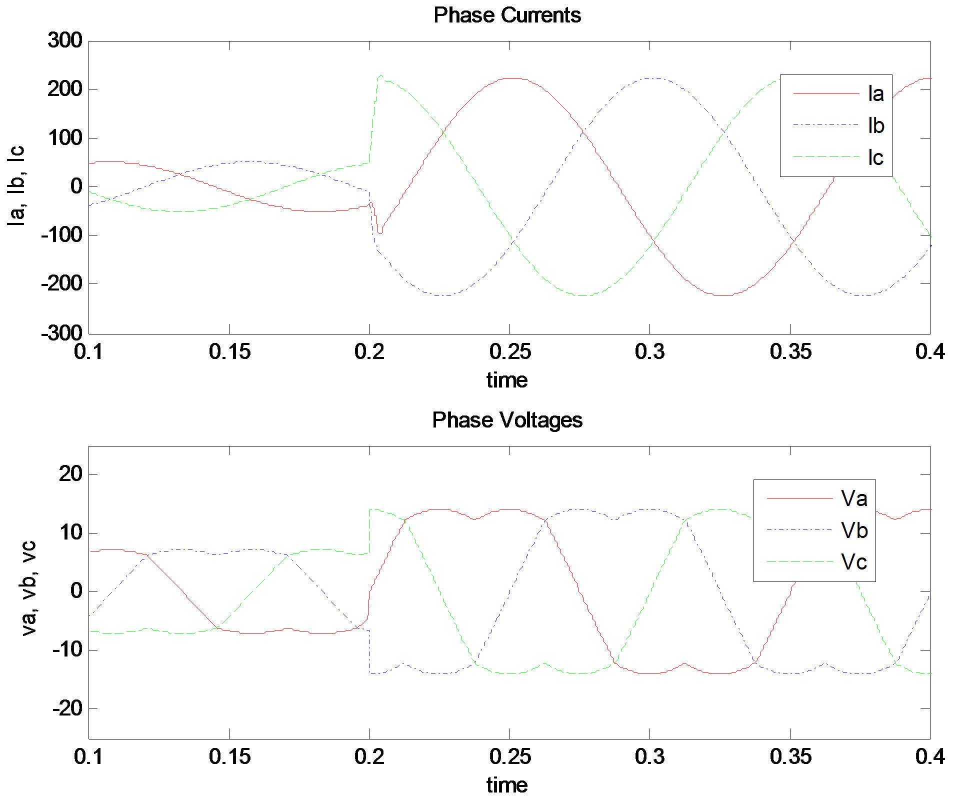
Figures 11(a)-(c) show the phase currents and phase voltages when the CLF method, the feedback linearization, and the PI controller methods are used respectively.
 (a)
(a)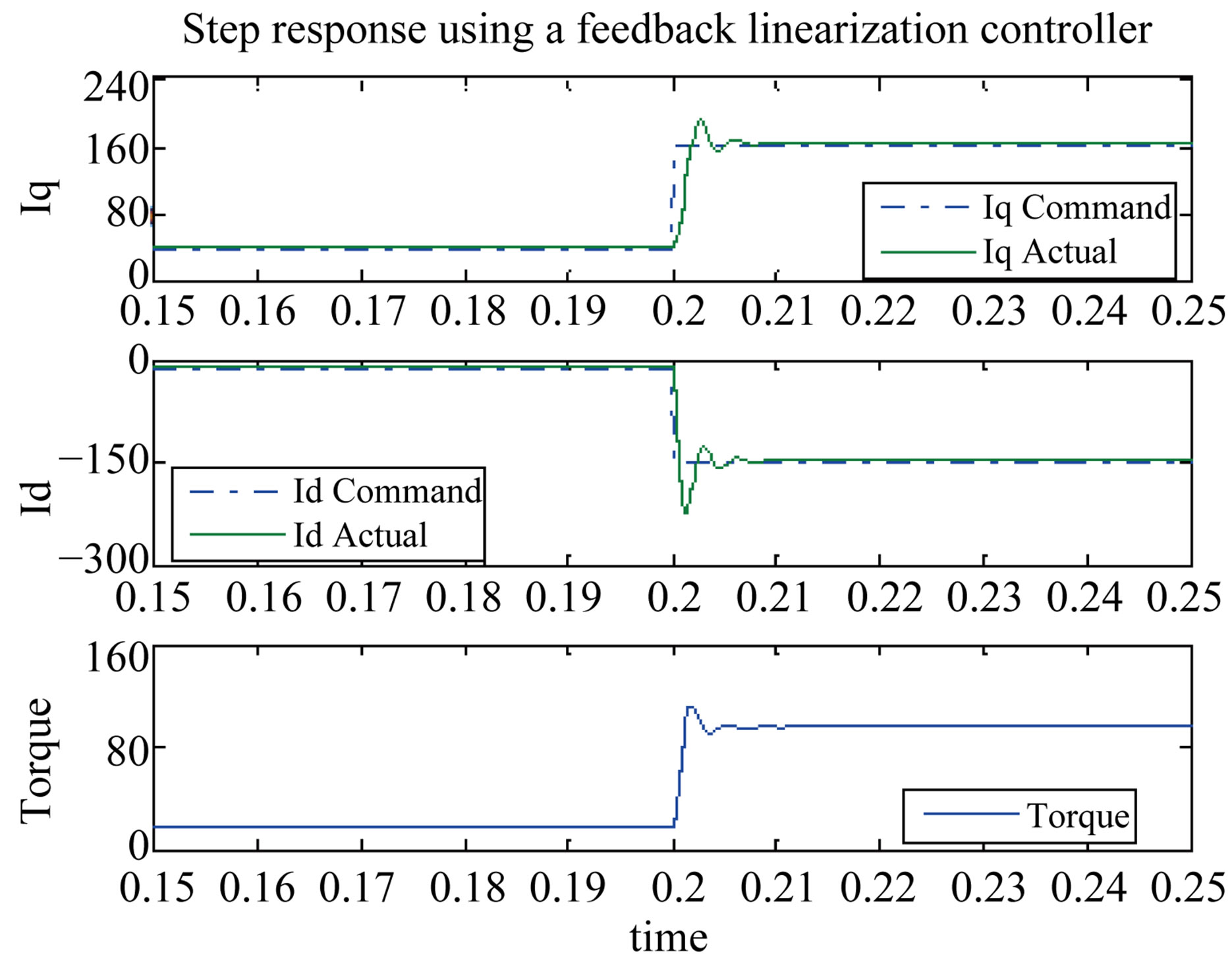 (b)
(b)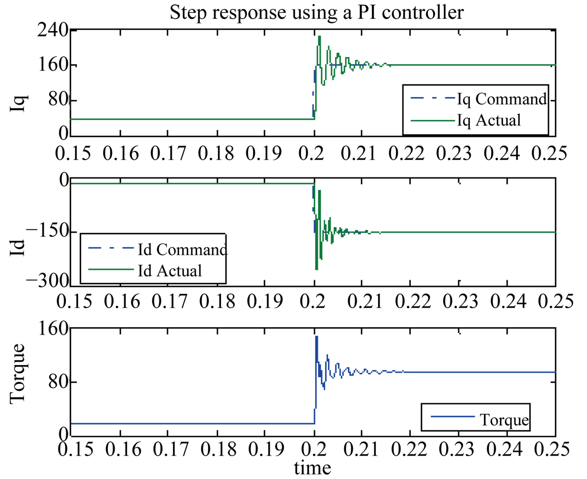 (c)
(c)
Figure 9. Torque and current response (2000 rpm). (a) CLF; (b) Feedback linearization; (c) PI controller.
The overshoots and oscillations in the step response will result in over currents and distortion of the sinusoidal current waveforms.
 (a)
(a)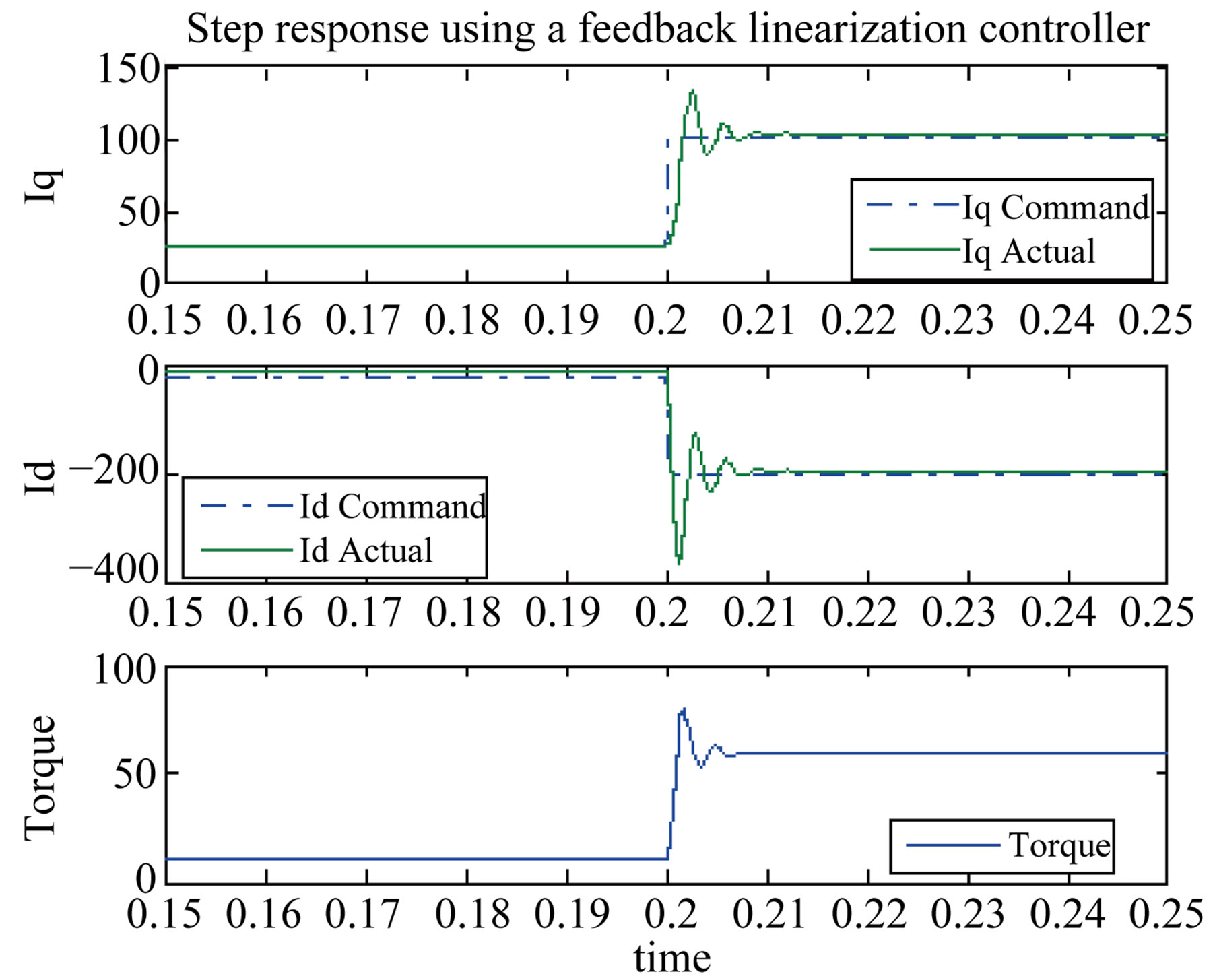 (b)
(b)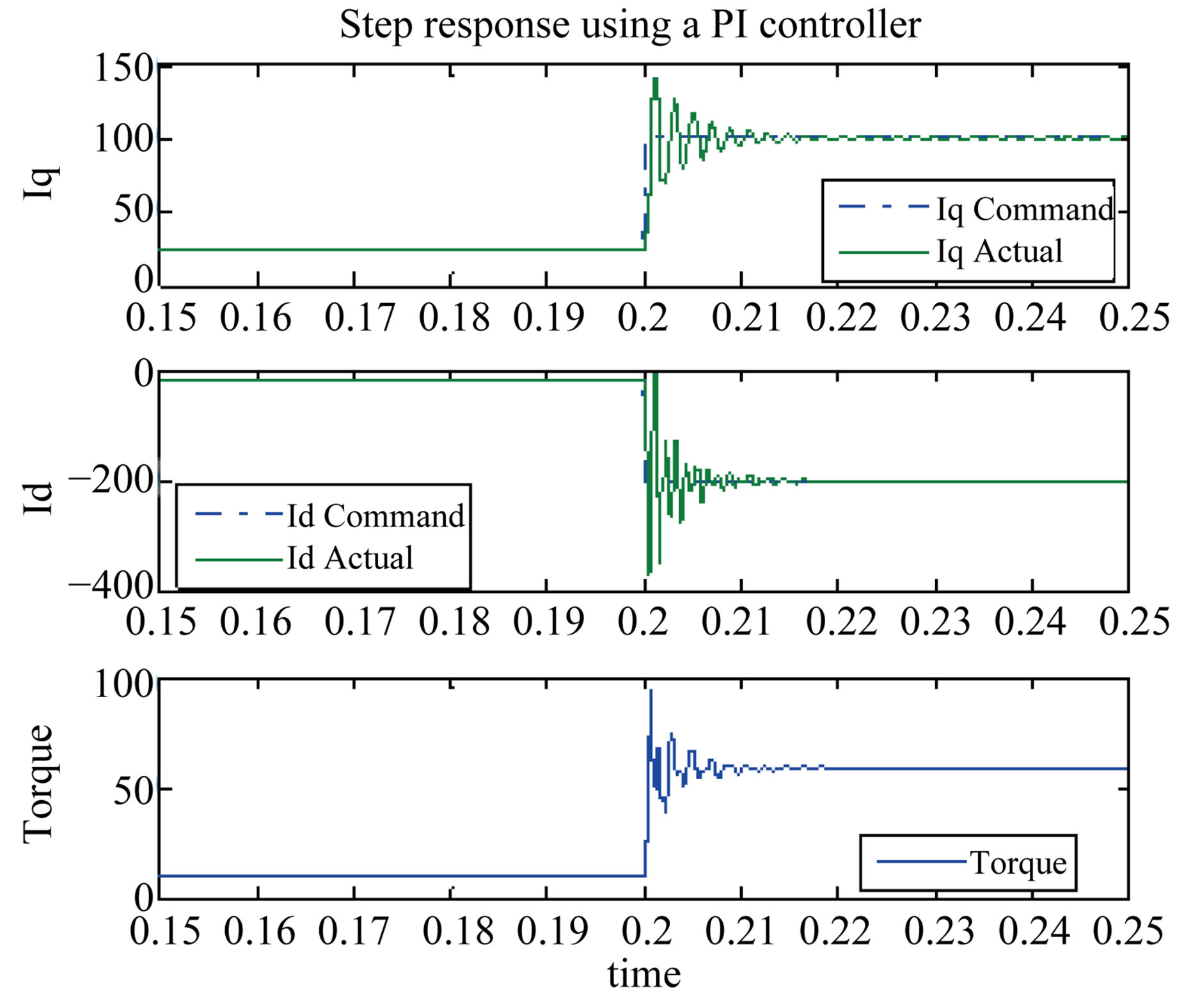 (c)
(c)
Figure 10. Torque and current response (4000 rpm). (a) CLF; (b) Feedback linearization; (c) PI controller.
6. Conclusion
The proposed nonlinear control for an interior permanent-magnet synchronous motor (IPMSM) for automo-
 (a)
(a)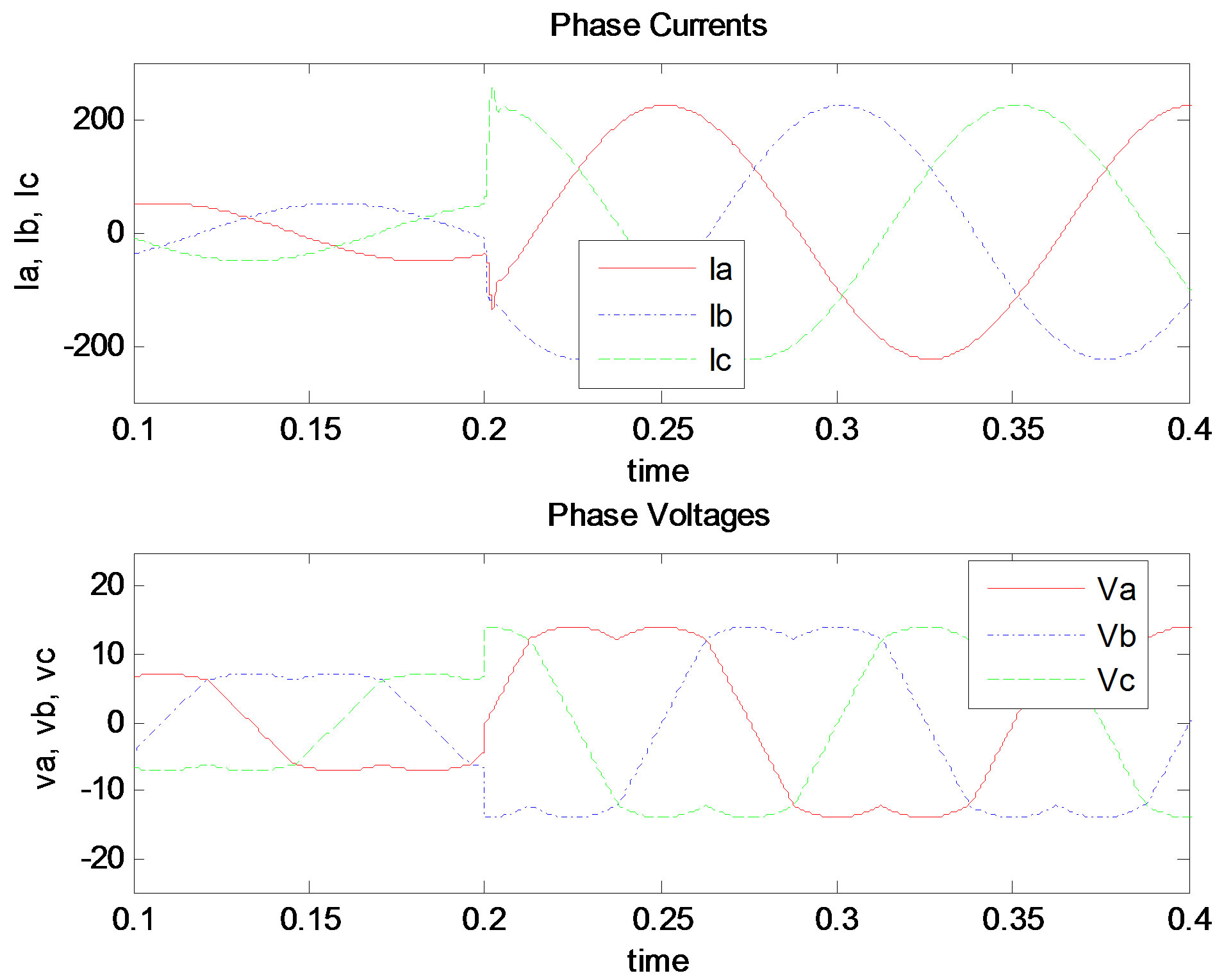 (b)
(b) (c)
(c)
Figure 11. Phase currents and phase voltages. (a) CLF; (b) Feedback linearization; (c) PI controller.
tive applications was presented. The method was shown to be stable and robust. Unlike the backstepping technique used in [1], the Control Lyapunov method proved effective in all operating regions. The authors in [1] made the assumption that id = 0 which was not realistic in an automotive application where it was necessary to operate along the most efficient trajectory in region I as shown in Figure 7. It is also necessary to operate in the flux weakening. The proposed method takes the system nonlinearities into account in the control system design stage while operating in the most efficient regions even in the flux weakening area. The nonlinearities that are taken into account are due to the cross coupling between the d and the q currents in addition to the system parameters. The motor parameters, which are a very important part in the control such as the flux linkages and inductances, are determined experimentally. In addition, the complete IPMSM drive incorporating the proposed CLF has been successfully simulated in a plant model for both motor and inverter and compared to a feedback linearization controller and to a conventional PI controller. The performance of the proposed drive was investigated in simulation at different operating conditions. It is found that the proposed control technique provides a good torque control performance for the IPMSM drive with no oscillations or overshoots while ensuring global stability. Tuning of the proposed method is also straightforward compared to the feedback linearization and the conventional PI control. In later work, we are planning to investigate other phenomena such as magnetic saturation, nonlinear loads, mechanical friction and flexibilities. In addition, efforts are being made to incorporate disturbances, quantitative robustness and diagnosis of faults into the future of control schemes.
REFERENCES
- M. A. Rahman, D. M. Vilathgamuwa, M. N. Uddin and K.-J. Tseng, “Nonlinear Control of Interior PermanentMagnet Synchronous Motor,” IEEE Transactions on Industry Applications, Vol. 39, No. 2, 2003, pp. 408-416. http://dx.doi.org/10.1109/TIA.2003.808932
- J. Solsona, M. I. Valla and C. Muravchik, “Nonlinear Control of a Permanent Magnet Synchronous Motor with Disturbance Torque Estimation,” IEEE Transactions on Energy Conversion, Vol. 15, No. 2, 2000, pp. 163-168. http://dx.doi.org/10.1109/60.866994
- G. S. Lakshmi, S. Kamakshaiah and T. R. Das, “Closed Loop PI Control of PMSM for Hybrid Electric Vehicle Using Three Level Diode Clamped Inverter for Optimal Efficiency,” International Conference on Energy Efficient Technologies for Sustainability (ICEETS), Nagercoil, 10- 12 April 2013, pp. 754-759. http://dx.doi.org/10.1109/ICEETS.2013.6533479
- J. Espina, A. Arias, J. Balcells and C. Ortega, “Speed Anti-Windup PI Strategies Review for Field Oriented Control of Permanent Magnet Synchronous Machines,” Compatibility and Power Electronics, Badajoz, 20-22 May 2009, pp. 279-285. http://dx.doi.org/10.1109/CPE.2009.5156047
- P. March and M. C. Turner, “Anti-Windup Compensator Designs for Nonsalient Permanent-Magnet Synchronous Motor Speed Regulators,” IEEE Transactions on Industry Applications, Vol. 45, No. 5, 2009, pp. 1598-1609. http://dx.doi.org/10.1109/TIA.2009.2027157
- J. L. Gao and Y. F. Zhang, “Research on Parameter Identification and PI Self-Tuning of PMSM,” 2nd International Conference on Information Science and Engineering (ICISE), Hangzhou, 4-6 December 2010, pp. 5251- 5254. http://dx.doi.org/10.1109/ICISE.2010.5690898
- R. G. Kanojiya and P. M. Meshram, “Optimal Tuning of PI Controller for Speed Control of DC Motor Drive Using Particle Swarm Optimization,” International Conference on Advances in Power Conversion and Energy Technologies (APCET), Mylavaram, 2-4 August 2012, pp. 1-6. http://dx.doi.org/10.1109/APCET.2012.6302000
- P. Pillay and R. Krishnan, “Modeling, Simulation, and Analysis of Permanent-Magnet Motor Drives. II. The Brushless DC Motor Drive,” IEEE Transactions on Industry Applications, Vol. 25, No. 2, 1989, pp. 274-279.
- A. Bacciotti and L. Rosier, “Liapunov Functions and Stability in Control Theory,” Springer-Verlag, London, 2001, pp. 119-154.
- H. K. Khalil, “Nonlinear Systems,” Prentice Hall, Upper Saddle River, 2002, pp. 111-161.
- E. Sontag, “A Lyapunov-Like Characterization of Asymptotic Controllability,” SIAM Journal on Control and Optimization, Vol. 21, No. 3, 1983, pp. 462-471. http://dx.doi.org/10.1137/0321028
- F. H. Clarke, Y. S. Ledyaev, E. D. Sontag and A. I. Subbotin, “Asymptotic Controllability Implies Feedback Stabilization,” IEEE Transactions on Automatic Control, Vol. 42, No. 10, 1997, pp. 1394-1407. http://dx.doi.org/10.1109/9.633828
- F. A. Alazabi and M. A. Zohdy, “Nonlinear Uncertain HIV-1 Model Controller by Using Control Lyapunov Function,” International Journal of Modern Nonlinear Theory and Application, Vol. 1, No. 2, 2012, pp. 33-39. http://dx.doi.org/10.4236/ijmnta.2012.12004
- M. Pahlevaninezhad, P. Das, J. Drobnik, G. Moschopoulos, P. K. Jain and A. Bakhshai, “A Nonlinear Optimal Control Approach Based on the Control-Lyapunov Function for an AC/DC Converter Used in Electric Vehicles,” IEEE Transactions on Industrial Informatics, Vol. 8, No. 3, 2012, pp. 596-614. http://dx.doi.org/10.1109/TII.2012.2193894