Asymptotic Stability of the Dynamic Solution of an N-Unit Series System with Finite Number of Vacations

doi:10.4236/jamp.2018.611185

Journal of Applied Mathematics and Physics
Vol.06 No.11(2018), Article ID:88423,17 pages
10.4236/jamp.2018.611185

Abdugeni Osman¹, Abdukerim Haji^1*, Askar Ablimit²

●How to Cite this Article

¹College of Mathematics and System Sciences, Xinjiang University, Urumqi, China

²School of Mathematics and Physics, Xinjiang Education Institute, Urumqi, China

This work is licensed under the Creative Commons Attribution International License (CC BY 4.0).

http://creativecommons.org/licenses/by/4.0/

Received: October 4, 2018; Accepted: November 10, 2018; Published: November 13, 2018

ABSTRACT

We investigate an N-unit series system with finite number of vacations. By analyzing the spectral distribution of the system operator and taking into account the irreducibility of the semigroup generated by the system operator we prove that the dynamic solution converges strongly to the steady state solution. Thus we obtain asymptotic stability of the dynamic solution of the system.

Keywords:

N-Unit Series System, C₀-Semigroup, Irreducibility, Asymptotic Stability

1. Introduction

The series repairable systems are the classical repairable systems in reliability theory. As a result of the strong practical background of series repairable systems, many researchers have studied them extensively under varying assumptions (see [1] [2] [3] [4] ). In [4] , the authors studied an N-unit series system with finite number of vacations and obtained some reliability expressions such as the Laplace transform of the reliability, the mean time to the first failure, the availability and the failure frequency of the system by using the supplementary variable method and the generalized Markov progress method as well as the Laplace transform. The authors used the dynamic solution and its asymptotic stability in calculating the availability and the reliability. But they did not prove the existence of the dynamic solution and the asymptotic stability of the dynamic solution. Motivated by this, A. Osman and A. Haji proved in [5] the existence of a unique positive dynamic solution of the system by using C₀-semigroup theory of linear operators. In this paper, we further study this system and prove that the dynamic solution of the system converges strongly to its steady state solution by analyzing the spectral distribution of the system operator and taking into account the irreducibility of the semigroup generated by the system operator; thus we obtain the asymptotic stability of the dynamic solution of this system.

The rest of this paper is organized as follows: In Section 2, we present the mathematical model of the system and give some results obtained in [5] . In Section 3, we obtain main result on stability of the system by analyzing the spectral distribution of the system operator and taking into account the irreducibility of the semigroup generated by the system operator.

2. Previous Results

According to [4] , the N-unit series system with finite number of vacations can be described by the following integro-differential equations:

${\begin{cases} (\frac{d}{d t} + Λ) p_{0} (t) = \int_{0}^{+ \infty} r (ω) p_{0 M} (t, ω) d ω, \\ (\frac{\partial}{\partial t} + \frac{\partial}{\partial y} + μ_{k} (y)) p_{k} (t, y) = 0, k = 1, 2, \dots, n, \\ (\frac{\partial}{\partial t} + \frac{\partial}{\partial ω} + r (ω)) p_{k j} (t, ω) = λ_{i} p_{0 j} (t, ω), k = 1, 2, \dots, n, j = 1, 2, \dots, M, \\ (\frac{\partial}{\partial t} + \frac{\partial}{\partial ω} + Λ + r (ω)) p_{0 j} (t, ω) = 0, j = 1, 2, \dots, M, \end{cases}$ (1)

With the boundary conditions

${\begin{cases} p_{k} (t, 0) = λ_{k} p_{0} (t) + \sum_{j = 1}^{M} \int_{0}^{\infty} r (ω) p_{k j} (t, ω) d ω, k = 1, 2, \dots, n, \\ p_{k j} (t, 0) = 0, k = 1, 2, \dots, n, j = 1, 2, \dots, M, \\ p_{01} (t, 0) = \sum_{k = 1}^{n} \int_{0}^{\infty} μ_{k} (y) p_{k} (t, y) d y, \\ p_{0 j} (t, 0) = \int_{0}^{\infty} r (ω) p_{0, j - 1} (t, ω) d ω, j = 2, \dots, M, \end{cases}$ (2)

and the initial conditions

${\begin{cases} p_{0} (0, ω) = 1, \\ p_{k} (0, y) = 0, k = 1, 2, \dots, n, \\ p_{k j} (0, ω) = 0, k = 1, 2, \dots, n, j = 1, 2, \dots, M \\ p_{0 j} (0, ω) = 0, j = 1, 2, \dots, M, \end{cases}$ (3)

where $Λ = λ_{1} + λ_{2} + \dots + λ_{n}$ .

Here $(t, y) \in [0, \infty) \times [0, \infty)$ ; $(t, ω) \in [0, \infty) \times [0, \infty)$ and the symbols in the equations have the following meaning.

$p_{0} (t)$ : The probability that n units at time t are in working state and the repairman is idle;

$p_{k} (t, y) d y$ : The probability that at time t the repairman is repairing the failed unit $k (k = 1, 2, \dots, n)$ , the elapsed repair time lies in $[y, y + d y)$ ;

$p_{0 j} (t, ω) d ω$ : The probability that n units at time t are in working state, the repairman is in $j (j = 1, 2, \dots, M)$ vacation and the elapsed repair time lies in $[ω, ω + d ω)$ ;

$p_{k j} (t, ω) d ω$ : The probability that at time t unit $k (k = 1, 2, \dots, n)$ is waiting for repair, the repairman is in $j (j = 1, 2, \dots, M)$ vacation and the elapsed repair time lies in $[ω, ω + d ω)$ ;

$λ_{k} (k = 1, 2, \dots, n)$ is positive constant; $r (ω)$ is the vacation rate function of the repairman;

$μ_{k} (y)$ is the repair rate function of unit k $(k = 1, 2, \dots, n)$ .

Throughout the paper we require the following assumption for the vacation rate function $r (ω)$ and the repair rate functions $μ_{k} (y) (k = 1, 2, \dots, n)$ .

General Assumption 2.1: The functions $r (ω)$ and $μ_{k} (y)$ : $[0, + \infty) \to [0, + \infty)$ $(k = 1, 2, \dots, n)$ are measurable and bounded such that

$r = \lim_{ω \to + \infty} r (ω) > 0, μ_{k} = \lim_{y \to + \infty} μ_{k} (y) > 0, μ_{\infty} = \min (r, μ_{k}) (k = 1, 2, \dots, n) .$ (4)

In [5] , the authors transformed the system (1), (2) and (3) into the following abstract Cauchy problem ( [6] , Def.II.6.1) on the Banach space $(X, ‖ \cdot ‖)$ .

${\begin{cases} \frac{d p (t)}{d t} = A p (t), t \in [0, + \infty), \\ p (0) = {(1, 0, 0, \dots, 0)}^{T} \in X, \end{cases}$ (5)

where

$X = ℂ \times {(L_{y}^{1} [0, + \infty))}^{n} \times {(L_{ω}^{1} [0, + \infty))}^{(n + 1) \times M}$ with norm

$‖ p ‖ = | p_{0} | + \sum_{i = 1}^{n} {‖ p_{i} ‖}_{L_{y}^{1} [0, + \infty)} + \sum_{i = 1}^{n} \sum_{1 = 1}^{M} {‖ p_{i j} ‖}_{L_{ω}^{1} [0, + \infty)} + \sum_{1 = 1}^{M} {‖ p_{0 j} ‖}_{L_{ω}^{1} [0, + \infty)}$ (6)

$\begin{array}{l} p = (p_{0}, p_{1} (y), p_{2} (y), \dots, p_{n} (y), p_{11} (ω), p_{12} (ω), \dots, p_{1 M} (ω), \\ p_{21} (ω), p_{22} (ω), \dots, p_{2 M} (ω), \dots, p_{n 1} (ω), p_{n 2} (ω), \dots, p_{n M} (ω), \\ p_{01} (ω), p_{02} (ω), \dots, {p_{0 M} (ω))}^{T} \in X, \end{array}$ (7)

$A p = A_{m} p, D (A) = {p \in D (A_{m}) | L p = Φ p}$ ,

(8)

$φ_{M} : f \mapsto φ_{M} (f) = \int_{0}^{+ \infty} r (ω) f (ω) d ω,$ (9)

$D_{i} = - \frac{d}{d y} - μ_{i} (y), k = 1, 2, \dots, n,$ (10)

$D_{k j} = - \frac{d}{d ω} - r (ω), k = 1, 2, \dots, n, j = 1, 2, \dots, M,$ (11)

$D_{0 j} = - [\frac{d}{d ω} + Λ + r (ω)], j = 1, 2, \dots, M,$ (12)

$L : D (A_{m}) \to \partial X, (\begin{matrix} p_{0} \\ p_{1} (y) \\ p_{2} (y) \\ ⋮ \\ p_{n} (y) \\ p_{11} (ω) \\ p_{12} (ω) \\ ⋮ \\ p_{1 M} (ω) \\ p_{21} (ω) \\ p_{22} (ω) \\ ⋮ \\ p_{2 M} (ω) \\ ⋮ \\ p_{n 1} (ω) \\ p_{n 2} (ω) \\ ⋮ \\ p_{n M} (ω) \\ p_{01} (ω) \\ p_{02} (ω) \\ ⋮ \\ p_{0 M} (ω) \end{matrix}) \to L (\begin{matrix} p_{0} \\ p_{1} (y) \\ p_{2} (y) \\ ⋮ \\ p_{n} (y) \\ p_{11} (ω) \\ p_{12} (ω) \\ ⋮ \\ p_{1 M} (ω) \\ p_{21} (ω) \\ p_{22} (ω) \\ ⋮ \\ p_{2 M} (ω) \\ ⋮ \\ p_{n 1} (ω) \\ p_{n 2} (ω) \\ ⋮ \\ p_{n M} (ω) \\ p_{01} (ω) \\ p_{02} (ω) \\ ⋮ \\ p_{0 M} (ω) \end{matrix}) = (\begin{matrix} p_{1} (0) \\ p_{2} (0) \\ ⋮ \\ p_{n} (0) \\ p_{11} (0) \\ p_{12} (0) \\ ⋮ \\ p_{1 M} (0) \\ p_{21} (0) \\ p_{22} (0) \\ ⋮ \\ p_{2 M} (0) \\ ⋮ \\ p_{n 1} (0) \\ p_{n 2} (0) \\ ⋮ \\ p_{n M} (0) \\ p_{01} (0) \\ p_{02} (0) \\ ⋮ \\ p_{0 M} (0) \end{matrix})$ (13)

$Φ L X \to \partial X, (\begin{matrix} p_{0} \\ p_{1} (y) \\ p_{2} (y) \\ ⋮ \\ p_{n} (y) \\ p_{11} (ω) \\ p_{12} (ω) \\ ⋮ \\ p_{1 M} (ω) \\ p_{21} (ω) \\ p_{22} (ω) \\ ⋮ \\ p_{2 M} (ω) \\ ⋮ \\ p_{n 1} (ω) \\ p_{n 2} (ω) \\ ⋮ \\ p_{n M} (ω) \\ p_{01} (ω) \\ p_{02} (ω) \\ ⋮ \\ p_{0 M} (ω) \end{matrix}) \to Φ (\begin{matrix} p_{0} \\ p_{1} (y) \\ p_{2} (y) \\ ⋮ \\ p_{n} (y) \\ p_{11} (ω) \\ p_{12} (ω) \\ ⋮ \\ p_{1 M} (ω) \\ p_{21} (ω) \\ p_{22} (ω) \\ ⋮ \\ p_{2 M} (ω) \\ ⋮ \\ p_{n 1} (ω) \\ p_{n 2} (ω) \\ ⋮ \\ p_{n M} (ω) \\ p_{01} (ω) \\ p_{02} (ω) \\ ⋮ \\ p_{0 M} ( ω ) \end{matrix})$

(14)

$φ_{k j} : f \mapsto φ_{k j} (f) = \int_{0}^{+ \infty} r (ω) f_{k j} (ω) d ω, k = 1, 2, \dots, n, j = 1, 2, \dots, M$ (15)

$φ_{k} : f \mapsto φ_{k} (f) = \int_{0}^{+ \infty} μ_{k} (y) f_{k} (y) d y, k = 1, 2, \dots, n,$ (16)

$φ_{0 j} : f \mapsto φ_{0 j} (f) = \int_{0}^{+ \infty} r (ω) f_{0 j - 1} (ω) d ω, j = 2, \dots, n$ (17)

and proved the following results.

Theorem 2.1: The operator $(A, D (A))$ generates a positive contraction C₀-semigroup ${(T (t))}_{t \geq 0}$ .

Theorem 2.2: The system (1), (2) and (3) has a unique positive dynamic solution

$\begin{array}{l} p (t) = (p_{0} (t), p_{1} (t, y), p_{2} (t, y), \dots, p_{n} (t, y), p_{11} (t, ω), p_{12} (t, ω), \dots, \\ p_{1 M} (t, ω), p_{21} (t, ω), p_{22} (t, ω), \dots, p_{2 M} (t, ω), \dots, p_{n 1} (t, ω), \\ p_{n 2} (t, ω), \dots, p_{n M} (t, ω), p_{01} (t, ω), p_{02} (t, ω), \dots, {p_{0 M} (t, ω))}^{T} \in X \end{array}$ (18)

which can be expressed as

$p (t) = T (t) p (0)$ . (19)

3. The Main Result

To prove our main result on the asymptotic stability of the dynamic solution of system, we first prove the some lemmas. In [7] , A. Haji and A. Radl gave the following result.

Lemma 3.1: Let $γ \in ρ (A_{0})$ , then

1) $γ \in σ_{p} (A) \Leftrightarrow 1 \in σ_{p} (Φ D_{γ})$ .

2) If $γ \in ρ (A_{0})$ and there exists $γ_{0} \in ℂ$ such that $1 \notin σ (Φ D_{γ_{0}})$ , then
$γ \in σ (A) \Leftrightarrow 1 \in σ (Φ D_{γ})$ .

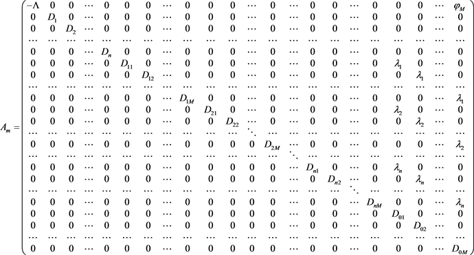
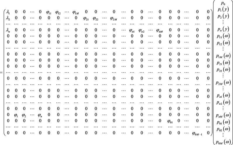
In our situation the operator $Φ D_{γ}$ is $(n + n \times M + M) \times (n + n \times M + M)$ -matrix, as follows:

$Φ D_{γ} = {\begin{matrix} 0 & 0 & \dots & 0 & a_{1, n + 1} & a_{1, n + 2} & \dots & a_{1, n + M} & 0 & 0 & \dots & 0 & \dots \\ 0 & 0 & \dots & 0 & 0 & 0 & \dots & 0 & a_{2, n + M + 1} & a_{2, n + M + 2} & \dots & a_{2, n + M + M} & \dots \\ \dots & \dots & \dots & \dots & \dots & \dots & \dots & \dots & \dots & \dots & \dots & \dots & \dots \\ 0 & 0 & \dots & 0 & 0 & 0 & \dots & 0 & 0 & 0 & \dots & 0 & \dots \\ 0 & 0 & \dots & 0 & 0 & 0 & \dots & 0 & 0 & 0 & \dots & 0 & \dots \\ 0 & 0 & \dots & 0 & 0 & 0 & \dots & 0 & 0 & 0 & \dots & 0 & \dots \\ \dots & \dots & \dots & \dots & \dots & \dots & \dots & \dots & \dots & \dots & \dots & \dots & \dots \\ 0 & 0 & \dots & 0 & 0 & 0 & \dots & 0 & 0 & 0 & \dots & 0 & \dots \\ 0 & 0 & \dots & 0 & 0 & 0 & \dots & 0 & 0 & 0 & \dots & 0 & \dots \\ 0 & 0 & \dots & 0 & 0 & 0 & \dots & 0 & 0 & 0 & \dots & 0 & \dots \\ \dots & \dots & \dots & \dots & \dots & \dots & \dots & \dots & \dots & \dots & ⋱ & \dots & \dots \\ 0 & 0 & \dots & 0 & 0 & 0 & \dots & 0 & 0 & 0 & \dots & 0 & \dots \\ \dots & \dots & \dots & \dots & \dots & \dots & ⋱ & \dots & \dots & \dots & \dots & \dots & ⋱ \\ 0 & 0 & \dots & 0 & 0 & 0 & \dots & 0 & 0 & 0 & \dots & 0 & \dots \\ 0 & 0 & \dots & 0 & 0 & 0 & \dots & 0 & 0 & 0 & \dots & 0 & \dots \\ \dots & \dots & \dots & \dots & \dots & \dots & \dots & \dots & \dots & \dots & \dots & \dots & \dots \\ 0 & 0 & \dots & 0 & 0 & 0 & \dots & 0 & 0 & 0 & \dots & 0 & \dots \\ a_{n + n M + 1, 1} & a_{n + n M + 1, 2} & \dots & a_{n + n M + 1, n} & 0 & 0 & \dots & 0 & 0 & 0 & \dots & 0 & \dots \\ 0 & 0 & \dots & 0 & 0 & 0 & \dots & 0 & 0 & 0 & \dots & 0 & \dots \\ \dots & \dots & \dots & \dots & \dots & \dots & \dots & \dots & \dots & \dots & \dots & \dots & \dots \\ 0 & 0 & \dots & 0 & 0 & 0 & \dots & 0 & 0 & 0 & \dots & 0 & \dots \end{matrix}$

$\begin{matrix} 0 & 0 & \dots & 0 & a_{1, n + n M + 1} & a_{1, n + n M + 2} & \dots & a_{1, n + n M + M - 1} & a_{1, n + n M + M} \\ 0 & 0 & \dots & 0 & a_{2, n + n M + 1} & a_{2, n + n M + 2} & \dots & a_{2, n + n M + M - 1} & a_{2, n + n M + M} \\ \dots & \dots & \dots & \dots & \dots & \dots & \dots & \dots & \dots \\ a_{n, n + (n - 1) M + 1} & a_{n, n + (n - 1) M + 2} & \dots & a_{n, n + n M} & a_{n, n + n M + 1} & a_{n, n + n M + 2} & \dots & a_{n, n + n M + M - 1} & a_{n, n + n M + M} \\ 0 & 0 & \dots & 0 & 0 & 0 & \dots & 0 & 0 \\ 0 & 0 & \dots & 0 & 0 & 0 & \dots & 0 & 0 \\ \dots & \dots & \dots & \dots & \dots & \dots & \dots & \dots & \dots \\ 0 & 0 & \dots & 0 & 0 & 0 & \dots & 0 & 0 \\ 0 & 0 & \dots & 0 & 0 & 0 & \dots & 0 & 0 \\ 0 & 0 & \dots & 0 & 0 & 0 & \dots & 0 & 0 \\ \dots & \dots & \dots & \dots & \dots & \dots & \dots & \dots & \dots \\ 0 & 0 & \dots & 0 & 0 & 0 & \dots & 0 & 0 \\ \dots & \dots & \dots & \dots & \dots & \dots & \dots & \dots & \dots \\ 0 & 0 & \dots & 0 & 0 & 0 & \dots & 0 & 0 \\ 0 & 0 & \dots & 0 & 0 & 0 & \dots & 0 & 0 \\ \dots & \dots & \dots & \dots & \dots & \dots & \dots & \dots & \dots \\ 0 & 0 & \dots & 0 & 0 & 0 & \dots & 0 & 0 \\ 0 & 0 & \dots & 0 & 0 & 0 & \dots & 0 & 0 \\ 0 & 0 & \dots & 0 & a_{n + n M + 2, n + n M + 1} & 0 & \dots & 0 & 0 \\ \dots & \dots & \dots & \dots & \dots & \dots & ⋱ & \dots & \dots \\ 0 & 0 & \dots & 0 & 0 & 0 & \dots & a_{n + n M + M, n + n M + M} & 0 \end{matrix}}$ (20)

where

$a_{n + n M + 1, 1} (γ) = \int_{0}^{+ \infty} μ_{1} (y) e^{- γ y - \int_{0}^{y} μ_{1} (t) d t} d y$ , $a_{n + n M + 1, 2} (γ) = \int_{0}^{+ \infty} μ_{2} (y) e^{- γ y - \int_{0}^{y} μ_{2} (t) d t} d y$ ,(21)

$\dots$ ,

$a_{n + n M + 1, n} (γ) = \int_{0}^{+ \infty} μ_{n} (y) e^{- γ y - \int_{0}^{y} μ_{n} (t) d t} d y$ , (22)

$a_{1, n + 1} (γ) = \int_{0}^{+ \infty} r (ω) e^{- γ ω - \int_{0}^{ω} r (s) d s} d ω$ , $a_{1, n + 2} (γ) = \int_{0}^{+ \infty} r (ω) e^{- γ ω - \int_{0}^{ω} r (s) d s} d ω$ , (23)

$\dots$ ,

$a_{1, n + M} (γ) = \int_{0}^{+ \infty} r (ω) e^{- γ ω - \int_{0}^{ω} r (s) d s} d ω$ , (24)

$a_{2, n + M + 1} (γ) = \int_{0}^{+ \infty} r (ω) e^{- γ ω - \int_{0}^{ω} r (s) d s} d ω$ , $a_{2, n + M + 2} (γ) = \int_{0}^{+ \infty} r (ω) e^{- γ ω - \int_{0}^{ω} r (s) d s} d ω$ ,(25)

$\dots$ ,

$a_{2, n + M + M} (γ) = \int_{0}^{+ \infty} r (ω) e^{- γ ω - \int_{0}^{ω} r (s) d s} d ω$ , $\dots$ , (26)

$a_{n, n + (n - 1) M + 1} (γ) = \int_{0}^{+ \infty} r (ω) e^{- γ ω - \int_{0}^{ω} r (s) d s} d ω$ ,

$a_{n, n + (n - 1) M + 2} (γ) = \int_{0}^{+ \infty} r (ω) e^{- γ ω - \int_{0}^{ω} r (s) d s} d ω$ , (27)

$\dots$ ,

$a_{n, n + n M} (γ) = \int_{0}^{+ \infty} r (ω) e^{- γ ω - \int_{0}^{ω} r (s) d s} d ω$ (28)

$a_{1, n + n M + 1} (γ) = \frac{λ_{1}}{Λ} \int_{0}^{+ \infty} r (ω) e^{- γ ω - \int_{0}^{ω} r (s) d s} (1 - e^{- Λ ω}) d ω$ , (29)

$a_{2, n + n M + 1} (γ) = \frac{λ_{2}}{Λ} \int_{0}^{+ \infty} r (ω) e^{- γ ω - \int_{0}^{ω} r (s) d s} (1 - e^{- Λ ω}) d ω$ , (30)

$\dots$ ,

$a_{n, n + n M + 1} (γ) = \frac{λ_{n}}{Λ} \int_{0}^{+ \infty} r (ω) e^{- γ ω - \int_{0}^{ω} r (s) d s} (1 - e^{- Λ ω}) d ω$ , (31)

$a_{n + n M + 2, n + n M + 1} (γ) = \int_{0}^{\infty} r (ω) e^{- γ ω - \int_{0}^{ω} r (s) d s} d ω$ , (32)

$a_{1, n + n M + 2} (γ) = \frac{λ_{1}}{Λ} \int_{0}^{+ \infty} r (ω) e^{- γ ω - \int_{0}^{ω} r (s) d s} (1 - e^{- Λ ω}) d ω$ , (33)

$a_{2, n + n M + 2} (γ) = \frac{λ_{2}}{Λ} \int_{0}^{+ \infty} r (ω) e^{- γ ω - \int_{0}^{ω} r (s) d s} (1 - e^{- Λ ω}) d ω$ , (34)

$\dots$ ,

$a_{n, n + n M + 2} (γ) = \frac{λ_{n}}{Λ} \int_{0}^{+ \infty} r (ω) e^{- γ ω - \int_{0}^{ω} r (s) d s} (1 - e^{- Λ ω}) d ω$ , (35)

$a_{n + n M + 3, n + n M + 2} (γ) = \int_{0}^{+ \infty} r (ω) e^{- γ ω - Λ ω - \int_{0}^{ω} r (s) d s} d ω$ , (36)

$\dots$ ,

$a_{1, n + n M + M - 1} (γ) = \frac{λ_{1}}{Λ} \int_{0}^{+ \infty} r (ω) e^{- γ ω - \int_{0}^{ω} r (s) d s} (1 - e^{- Λ ω}) d ω$ , (37)

$a_{2, n + n M + M - 1} (γ) = \frac{λ_{2}}{Λ} \int_{0}^{+ \infty} r (ω) e^{- γ ω - \int_{0}^{ω} r (s) d s} (1 - e^{- Λ ω}) d ω$ , (38)

$\dots$ ,

$a_{n, n + n M + M - 1} (γ) = \frac{λ_{n}}{Λ} \int_{0}^{+ \infty} r (ω) e^{- γ ω - \int_{0}^{ω} r (s) d s} (1 - e^{- Λ ω}) d ω$ , (39)

$a_{n + n M + M, n + n M + M - 1} (γ) = \int_{0}^{+ \infty} r (ω) e^{- γ ω - Λ ω - \int_{0}^{ω} r (s) d s} d ω$ , (40)

$\begin{matrix} a_{1, n + n M + M} (γ) = \frac{λ_{1}}{Λ} \int_{0}^{\infty} r (ω) e^{- γ ω - Λ ω - \int_{0}^{ω} r (s) d s} d ω \\ + \frac{λ_{1}}{Λ} \int_{0}^{\infty} r (ω) e^{- γ ω - \int_{0}^{ω} r (s) d s} (1 - e^{- Λ ω}) d ω \end{matrix}$ , (41)

$\begin{matrix} a_{2, n + n M + M} (γ) = \frac{λ_{2}}{Λ} \int_{0}^{\infty} r (ω) e^{- γ ω - Λ ω - \int_{0}^{ω} r (s) d s} d ω \\ + \frac{λ_{2}}{Λ} \int_{0}^{\infty} r (ω) e^{- γ ω - \int_{0}^{ω} r (s) d s} (1 - e^{- Λ ω}) d ω \end{matrix}$ , (42)

$\dots$ ,

$\begin{matrix} a_{n, n + n M + M} (γ) = \frac{λ_{n}}{Λ} \int_{0}^{\infty} r (ω) e^{- γ ω - Λ ω - \int_{0}^{ω} r (s) d s} d ω \\ + \frac{λ_{n}}{Λ} \int_{0}^{\infty} r (ω) e^{- γ ω - \int_{0}^{ω} r (s) d s} (1 - e^{- Λ ω}) d ω \end{matrix}$ . (43)

Lemma 3.2: For the operator $(A, D (A))$ we have $0 \in σ_{p} (A)$ .

Proof: All the entries of $Φ D_{0}$ are positive and one can compute each column sum of the $(n + n \times M + M) \times (n + n \times M + M)$ -matrix $Φ D_{0}$ as follows.

$\begin{array}{l} a_{1, 1} (0) + a_{2, 1} (0) + \dots + a_{n + n M + 1, 1} (0) + \dots + a_{n + n M + M, 1} (0) \\ = a_{n + n M + 1, 1} (0) = \int_{0}^{+ \infty} μ_{1} (y) e^{- \int_{0}^{y} μ_{1} (t) d t} d y = 1 \end{array}$ , (44)

$\begin{array}{l} a_{1, 2} (0) + a_{2, 2} (0) + \dots + a_{n + n M + 1, 2} (0) + \dots + a_{n + n M + M, 2} (0) \\ = a_{n + n M + 1, 2} (0) = \int_{0}^{+ \infty} μ_{2} (y) e^{- \int_{0}^{y} μ_{2} (t) d t} d y = 1 \end{array}$ , (45)

$\dots$

$\begin{array}{l} a_{1, n} (0) + a_{2, n} (0) + \dots + a_{n + n M + 1, n} (0) + \dots + a_{n + n M + M, n} (0) \\ = a_{n + n M + 1, n} (0) = \int_{0}^{+ \infty} μ_{n} (y) e^{- \int_{0}^{y} μ_{n} (t) d t} d y = 1 \end{array}$ , (46)

$\begin{array}{l} a_{1, n + 1} (0) + a_{2, n + 1} (0) + \dots + a_{n + n M + M, n + 1} (0) \\ = a_{1, n + 1} (0) = \int_{0}^{+ \infty} r (ω) e^{- \int_{0}^{ω} r (s) d s} d ω = 1 \end{array}$ , (47)

$\begin{array}{l} a_{1, n + 2} (0) + a_{2, n + 2} (0) + \dots + a_{n + n M + M, n + 2} (0) \\ = a_{1, n + 2} (0) = \int_{0}^{+ \infty} r (ω) e^{- \int_{0}^{ω} r (s) d s} d ω = 1 \end{array}$ , (48)

$\dots$

$\begin{array}{l} a_{1, n + M} (0) + a_{2, n + M} (0) + \dots + a_{n + n M + M, n + M} (0) \\ = a_{1, n + M} (0) = \int_{0}^{+ \infty} r (ω) e^{- \int_{0}^{ω} r (s) d s} d ω = 1 \end{array}$ , (49)

$\begin{array}{l} a_{1, n + M + 1} (0) + a_{2, n + M + 1} (0) + \dots + a_{n + n M + M, n + M + 1} (0) \\ = a_{2, n + M + 1} (0) = \int_{0}^{+ \infty} r (ω) e^{- \int_{0}^{ω} r (s) d s} d ω = 1 \end{array}$ , (50)

$\begin{array}{l} a_{1, n + M + 2} (0) + a_{2, n + M + 2} (0) + \dots + a_{n + n M + M, n + M + 2} (0) \\ = a_{2, n + M + 2} (0) = \int_{0}^{+ \infty} r (ω) e^{- \int_{0}^{ω} r (s) d s} d ω = 1 \end{array}$ , (51)

$\dots$

$\begin{array}{l} a_{1, n + M + M} (0) + a_{2, n + M + M} (0) + \dots + a_{n + n M + M, n + M + M} (0) \\ = a_{2, n + M + M} (0) = \int_{0}^{+ \infty} r (ω) e^{- \int_{0}^{ω} r (s) d s} d ω = 1 \end{array}$ , (52)

$\dots$

$\begin{array}{l} a_{1, n + (n - 1) M + 1} (0) + a_{2, n + (n - 1) M + 1} (0) + \dots + a_{n, n + (n - 1) M + 1} (0) + \dots + a_{n + n M + M, n + (n - 1) M + 1} (0) \\ = a_{n, n + (n - 1) M + 1} (0) = \int_{0}^{+ \infty} r (ω) e^{- \int_{0}^{ω} r (s) d s} d ω = 1 \end{array}$ , (53)

$\begin{array}{l} a_{1, n + (n - 1) M + 2} (0) + a_{2, n + (n - 1) M + 2} (0) + \dots + a_{n, n + (n - 1) M + 2} (0) + \dots + a_{n + n M + M, n + (n - 1) M + 2} (0) \\ = a_{n, n + (n - 1) M + 2} (0) = \int_{0}^{+ \infty} r (ω) e^{- \int_{0}^{ω} r (s) d s} d ω = 1 \end{array}$ , (54)

$\dots$

$\begin{array}{l} a_{1, n + n M} (0) + a_{2, n + n M} (0) + \dots + a_{n, n + n M} (0) + \dots + a_{n + n M + M, n + n M} (0) \\ = a_{n, n + n M} (0) = \int_{0}^{+ \infty} r (ω) e^{- \int_{0}^{ω} r (s) d s} d ω = 1 \end{array}$ , (55)

$\begin{array}{l} a_{1, n + n M + 1} (0) + a_{2, n + n M + 1} (0) + \dots + a_{n, n + n M + 1} (0) + \dots + a_{n + n M + 2, n + n M + 1} (0) + \dots \\ + a_{n + n M + M, n + n M + 1} (0) \\ = a_{1, n + n M + 1} (0) + a_{2, n + n M + 1} (0) + \dots + a_{n, n + n M + 1} (0) + \dots + a_{n + n M + 2, n + n M + 1} (0) \\ = \frac{λ_{1}}{Λ} \int_{0}^{+ \infty} r (ω) e^{- \int_{0}^{ω} r (s) d s} (1 - e^{- Λ ω}) d ω + \frac{λ_{2}}{Λ} \int_{0}^{+ \infty} r (ω) e^{- \int_{0}^{ω} r (s) d s} (1 - e^{- Λ ω}) d ω + \dots \\ + \frac{λ_{n}}{Λ} \int_{0}^{+ \infty} r (ω) e^{- \int_{0}^{ω} r (s) d s} (1 - e^{- Λ ω}) d ω + \int_{0}^{+ \infty} r (ω) e^{- Λ ω - \int_{0}^{ω} r (s) d s} d ω \end{array}$

$\begin{array}{l} = \int_{0}^{+ \infty} r (ω) e^{- \int_{0}^{ω} r (s) d s} (1 - e^{- Λ ω}) d ω + \int_{0}^{+ \infty} r (ω) e^{- Λ ω - \int_{0}^{ω} r (s) d s} d ω \\ = \int_{0}^{+ \infty} r (ω) e^{- \int_{0}^{ω} r (s) d s} d ω = 1 \end{array}$ , (56)

$\begin{array}{l} a_{1, n + n M + 2} (0) + a_{2, n + n M + 2} (0) + \dots + a_{n, n + n M + 2} (0) + \dots + a_{n + n M + 3, n + n M + 2} (0) + \dots \\ + a_{n + n M + M, n + n M + 2} (0) \\ = a_{1, n + n M + 2} (0) + a_{2, n + n M + 2} (0) + \dots + a_{n, n + n M + 2} (0) + \dots + a_{n + n M + 3, n + n M + 2} (0) \\ = \frac{λ_{1}}{Λ} \int_{0}^{+ \infty} r (ω) e^{- \int_{0}^{ω} r (s) d s} (1 - e^{- Λ ω}) d ω + \frac{λ_{2}}{Λ} \int_{0}^{+ \infty} r (ω) e^{- \int_{0}^{ω} r (s) d s} (1 - e^{- Λ ω}) d ω + \dots \\ + \frac{λ_{n}}{Λ} \int_{0}^{+ \infty} r (ω) e^{- \int_{0}^{ω} r (s) d s} (1 - e^{- Λ ω}) d ω + \int_{0}^{+ \infty} r (ω) e^{- Λ ω - \int_{0}^{ω} r (s) d s} d ω \end{array}$

$\dots$ ,

$\begin{array}{l} a_{1, n + n M + M - 1} (0) + a_{2, n + n M + M - 1} (0) + \dots + a_{n, n + n M + M - 1} (0) + \dots \\ + a_{n + n M + M, n + n M + M - 1} (0) + \dots + a_{n + n M + M, n + n M + M - 1} (0) \\ = a_{1, n + n M + M - 1} (0) + a_{2, n + n M + M - 1} (0) + \dots + a_{n, n + n M + M - 1} (0) + \dots + a_{n + n M + M, n + n M + M - 1} (0) \\ = \frac{λ_{1}}{Λ} \int_{0}^{+ \infty} r (ω) e^{- \int_{0}^{ω} r (s) d s} (1 - e^{- Λ ω}) d ω + \frac{λ_{2}}{Λ} \int_{0}^{+ \infty} r (ω) e^{- \int_{0}^{ω} r (s) d s} (1 - e^{- Λ ω}) d ω + \dots \\ + \frac{λ_{n}}{Λ} \int_{0}^{+ \infty} r (ω) e^{- \int_{0}^{ω} r (s) d s} (1 - e^{- Λ ω}) d ω + \int_{0}^{+ \infty} r (ω) e^{- Λ ω - \int_{0}^{ω} r (s) d s} d ω \end{array}$

$\begin{array}{l} a_{1, n + n M + M} (0) + a_{2, n + n M + M} (0) + \dots + a_{n, n + n M + M} (0) + \dots + a_{n + n M + M, n + n M + M} (0) \\ = a_{1, n + n M + M} (0) + a_{2, n + n M + M} (0) + \dots + a_{n, n + n M + M} (0) \\ = \frac{λ_{1}}{Λ} \int_{0}^{+ \infty} r (ω) e^{- Λ ω - \int_{0}^{ω} r (s) d s} d ω + \frac{λ_{1}}{Λ} \int_{0}^{+ \infty} r (ω) e^{- \int_{0}^{ω} r (s) d s} (1 - e^{- Λ ω}) d ω \\ + \frac{λ_{2}}{Λ} \int_{0}^{+ \infty} r (ω) e^{- Λ ω - \int_{0}^{ω} r (s) d s} d ω + \frac{λ_{2}}{Λ} \int_{0}^{+ \infty} r (ω) e^{- \int_{0}^{ω} r (s) d s} (1 - e^{- Λ ω}) d ω + \dots \\ + \frac{λ_{n}}{Λ} \int_{0}^{+ \infty} r (ω) e^{- Λ ω - \int_{0}^{ω} r (s) d s} d ω + \frac{λ_{n}}{Λ} \int_{0}^{+ \infty} r (ω) e^{- \int_{0}^{ω} r (s) d s} (1 - e^{- Λ ω}) d ω \\ = \int_{0}^{+ \infty} r (ω) e^{- \int_{0}^{ω} r (s) d s} d ω = 1 \end{array}$ . (59)

From these results we know that the matrix $Φ D_{0}$ is column stochastic and thus $1 \in σ_{p} (Φ D_{0})$ . Applying Lemma 3.1 1), we immediately obtain $0 \in σ_{p} (A)$ .

Using Lemma 3.1 2) we can show that 0 is the only spectral point of A on the imaginary axis.

Lemma 3.3: The spectrum $σ (A)$ of A satisfies

$σ (A) \cap i R = {0}$ . (60)

Proof: By Lemma 3.1 it suffices to prove that $a i \notin σ (Φ D_{a i})$ for all $a \in R$ , $a \neq 0$ .

Since the General Assumption 2.1 implies that there exists $r \in ℝ_{+}$ such that

$μ_{k} (y) > 0, k = 1, 2, \dots, n$ and $r (x) > 0$ for all $y, ω \in [r, r + \frac{2π}{a}]$ . Using the abbreviation $g (y) : = μ_{k} (y) e^{- \int_{0}^{y} μ_{k} (τ) d τ}, k = 1, 2, \dots, n$ we can estimate

$\begin{array}{l} | \int_{0}^{+ \infty} μ_{k} (y) e^{- a i y - \int_{0}^{y} μ_{k} (τ) d τ} d y | = | \int_{0}^{+ \infty} e^{- a i y} μ_{k} (y) e^{- \int_{0}^{y} μ_{k} (τ) d τ} d y | = | \int_{0}^{+ \infty} e^{- a i y} g (y) d y | \\ \leq | \int_{r}^{r + \frac{2π}{a}} e^{- a i y} g (y) d y | + | \int_{0}^{r} e^{- a i y} g (y) d y + \int_{r + \frac{2π}{a}}^{+ \infty} e^{- a i y} g (y) d y | \\ \leq | \int_{r}^{r + \frac{2π}{a}} e^{- a i y} g (y) d y | + \int_{0}^{r} g (y) d y + \int_{r + \frac{2π}{a}}^{+ \infty} g (y) d y, k = 1, 2, \dots, n \end{array}$ (61)

The first term on the right hand side of the inequality (61) can be estimated as

$\begin{array}{l} | \int_{r}^{r + \frac{2π}{a}} e^{- a i y} g (y) d y | = | \int_{r}^{r + \frac{π}{a}} e^{- a i y} g (y) d y + \int_{r + \frac{π}{a}}^{r + \frac{2π}{a}} e^{- a i y} g (y) d y | \\ = | \int_{r}^{r + \frac{π}{a}} e^{- a i y} g (y) d y + \int_{r}^{r + \frac{π}{a}} e^{- a i (y + \frac{π}{a})} g (y + \frac{π}{a}) d y | \\ = | \int_{r}^{r + \frac{π}{a}} e^{- a i y} g (y) d y + \int_{r}^{r + \frac{π}{a}} e^{- π i} e^{- a i y} g (y + \frac{π}{a}) d y | \\ = | \int_{r}^{r + \frac{π}{a}} e^{- a i y} [g (y) - g (y + \frac{π}{a})] d y | \leq \int_{r}^{r + \frac{π}{a}} | g (y) - g (y + \frac{π}{a}) | d y \\ < \int_{r}^{r + \frac{π}{a}} [g (y) + g (y + \frac{π}{a})] d y = \int_{r}^{r + \frac{π}{a}} g (y) d y + \int_{r + \frac{π}{a}}^{r + \frac{2π}{a}} g (y) d y = \int_{r}^{r + \frac{2π}{a}} g (y) d y, \end{array}$ (62)

where we used the strict positivity of $μ_{k} (y)$ on $[r, r + \frac{2 π}{a}]$ in the last inequality. By inserting (62) into (61) we have

$\begin{array}{l} | \int_{0}^{+ \infty} μ_{k} (y) e^{- a i y - \int_{0}^{y} μ_{k} (τ) d τ} d y | < \int_{r}^{r + \frac{2π}{a}} g (y) d y + \int_{0}^{r} g (y) d y + \int_{r + \frac{2π}{a}}^{+ \infty} g (y) d y \\ = \int_{0}^{+ \infty} g (y) d y = 1, k = 1, 2, \dots, n \end{array}$ (63)

Using the same way we can also estimate

$| \int_{0}^{+ \infty} r (ω) e^{- a i ω - \int_{0}^{ω} r (s) d s} d ω | < 1$ , (64)

$| \int_{0}^{+ \infty} r (ω) e^{- a i ω - \int_{0}^{ω} r (s) d s} (1 - e^{- Λ ω}) d ω | < \int_{0}^{+ \infty} r (ω) e^{- \int_{0}^{ω} r (s) d s} (1 - e^{- Λ ω}) d ω$ , (65)

$| \int_{0}^{+ \infty} r (ω) e^{- a i ω - Λ ω - \int_{0}^{ω} r (s) d s} d ω | < \int_{0}^{+ \infty} r (ω) e^{- Λ ω - \int_{0}^{ω} r (s) d s} d ω$ . (66)

Using (63)-(66) we can estimate each column sum of absolute entries of $Φ D_{a i}$ as follows.

$\begin{array}{l} | a_{1, k} (a i) | + | a_{2, k} (a i) | + \dots + | a_{n + n M + 1, k} (a i) | + \dots + | a_{n + n M + M, k} (a i) | \\ = | a_{a n + n M + 1, k} (a i) | = | \int_{0}^{+ \infty} μ_{k} (y) e^{- a i y - \int_{0}^{y} μ_{k} (τ) d τ} d y | < 1, k = 1, 2, \dots, n, \end{array}$ (67)

$\begin{array}{l} | a_{1, n + j} (a i) | + | a_{2, n + j} (a i) | + \dots + | a_{n + n M + 1, n + j} (a i) | + \dots + | a_{n + n M + M, n + j} (a i) | \\ = | a_{1, n + j} (a i) | = | \int_{0}^{+ \infty} μ_{k} (y) e^{- a i y - \int_{0}^{y} μ_{k} (τ) d τ} d y | < 1, j = 1, 2, \dots, M \end{array}$ (68)

$\begin{array}{l} | a_{1, n + M + j} (a i) | + | a_{2, n + M + j} (a i) | + \dots + | a_{n + n M + M, n + M + j} (a i) | \\ = | a_{2, n + M + j} (a i) | = | \int_{0}^{+ \infty} μ_{k} (y) e^{- a i y - \int_{0}^{y} μ_{k} (τ) d τ} d y | < 1, j = 1, 2, \dots, M, \end{array}$ (69)

$\dots$ ,

$\begin{array}{l} | a_{1, n + (n - 1) M + j} (a i) | + | a_{2, n + (n - 1) M + j} (a i) | + \dots + | a_{n, n + (n - 1) M + j} (a i) | \\ + \dots + | a_{n + n M + M, n + (n - 1) M + j} (a i) | \\ = | a_{n, n + (n - 1) M + j} (a i) | = | \int_{0}^{+ \infty} μ_{k} (y) e^{- a i y - \int_{0}^{y} μ_{k} (τ) d τ} d y | < 1, j = 1, 2, \dots, M, \end{array}$ (70)

$\begin{array}{l} | a_{1, n + n M + j} (a i) | + | a_{2, n + n M + j} (a i) | + \dots + | a_{n, n + n M + j} (a i) | + \dots \\ + | a_{n + n M + 2, n + n M + j} (a i) | + \dots + | a_{n + n M + M, n + n M + j} (a i) | \\ = | a_{1, n + n M + j} (a i) | + | a_{2, n + n M + j} (a i) | + \dots + | a_{n, n + n M + j} (a i) | + \dots + | a_{n + n M + 2, n + n M + j} (a i) | \\ = | \frac{λ_{1}}{Λ} \int_{0}^{+ \infty} r (ω) e^{- a i ω - \int_{0}^{ω} r (τ) d τ} (1 - e^{- Λ ω}) d ω | + | \frac{λ_{2}}{Λ} \int_{0}^{+ \infty} r (ω) e^{- a i ω - \int_{0}^{ω} r (τ) d τ} (1 - e^{- Λ ω}) d ω | \\ + \dots + | \frac{λ_{n}}{Λ} \int_{0}^{+ \infty} r (ω) e^{- a i ω - \int_{0}^{ω} r (τ) d τ} (1 - e^{- Λ ω}) d ω | + | \int_{0}^{+ \infty} r (ω) e^{- a i ω - Λ ω - \int_{0}^{ω} r (τ) d τ} d ω | \end{array}$

$\begin{array}{l} = | \int_{0}^{+ \infty} r (ω) e^{- a i ω - \int_{0}^{ω} r (τ) d τ} (1 - e^{- Λ ω}) d ω | + | \int_{0}^{+ \infty} r (ω) e^{- a i ω - Λ ω - \int_{0}^{ω} r (τ) d τ} d ω | \\ < \int_{0}^{+ \infty} r (ω) e^{- \int_{0}^{ω} r (τ) d τ} (1 - e^{- Λ ω}) d ω + \int_{0}^{+ \infty} r (ω) e^{- Λ ω - \int_{0}^{ω} r (τ) d τ} d ω \\ = \int_{0}^{+ \infty} r (ω) e^{- \int_{0}^{ω} r (τ) d τ} d ω = 1, j = 1, 2, \dots, M - 1, \end{array}$ (71)

$\begin{array}{l} | a_{1, n + n M + M} (a i) | + | a_{2, n + n M + M} (a i) | + \dots + | a_{n, n + n M + M} (a i) | + \dots + | a_{n + n M + M, n + n M + M} (a i) | \\ = | a_{1, n + n M + M} (a i) | + | a_{2, n + n M + M} (a i) | + \dots + | a_{n, n + n M + M} (a i) | \\ = | \frac{λ_{1}}{Λ} \int_{0}^{+ \infty} r (ω) e^{- a i ω - \int_{0}^{ω} r (τ) d τ} (1 - e^{- Λ ω}) d ω + \frac{λ_{1}}{Λ + a i} \int_{0}^{+ \infty} r (ω) e^{- (a i + Λ) ω - \int_{0}^{ω} r (τ) d τ} d ω | \\ + | \frac{λ_{2}}{Λ} \int_{0}^{+ \infty} r (ω) e^{- a i ω - \int_{0}^{ω} r (τ) d τ} (1 - e^{- Λ ω}) d ω + \frac{λ_{2}}{Λ + a i} \int_{0}^{+ \infty} r (ω) e^{- (a i + Λ) ω - \int_{0}^{ω} r (τ) d τ} d ω | \\ + \dots + | \frac{λ_{n}}{Λ} \int_{0}^{+ \infty} r (ω) e^{- a i ω - \int_{0}^{ω} r (τ) d τ} (1 - e^{- Λ ω}) d ω + \frac{λ_{n}}{Λ + a i} \int_{0}^{+ \infty} r (ω) e^{- (a i + Λ) ω - \int_{0}^{ω} r (τ) d τ} d ω | \end{array}$ $\begin{array}{l} \leq \int_{0}^{+ \infty} r (ω) e^{- \int_{0}^{ω} r (τ) d τ} (1 - e^{- Λ ω}) d ω + \frac{Λ}{Λ^{2} + a^{2}} \int_{0}^{+ \infty} r (ω) e^{- Λ ω - \int_{0}^{ω} r (τ) d τ} d ω \\ < \int_{0}^{+ \infty} r (ω) e^{- \int_{0}^{ω} r (τ) d τ} (1 - e^{- Λ ω}) d ω + \int_{0}^{+ \infty} r (ω) e^{- Λ ω - \int_{0}^{ω} r (τ) d τ} d ω \\ = \int_{0}^{+ \infty} r (ω) e^{- \int_{0}^{ω} r (τ) d τ} d ω = 1 \end{array}$ (72)

From (67)-(72) we deduce $‖ Φ D_{a i} ‖ < 1$ , thus the spectral radius fulfills $r (Φ D_{a i}) \leq ‖ Φ D_{a i} ‖ < 1$ . This implies $1 \in ρ (Φ D_{a i})$ for all $a \in R, a \neq 0$ , i.e. $a i \notin σ (Φ D_{a i})$ for all $a \in R, a \neq 0$ . By Lemma 3.1 2) we obtain that $a i \notin σ (A)$ for all $a \in R, a \neq 0$ , i.e., $σ (A) \cap i R = {0}$ .

Lemma 3.4: If the operator $(A_{0}, D (A_{0}))$ is defined as

$A_{0} p = A_{m} p, D (A_{0}) = {p \in D (A_{m}) | L p = 0},$ (73)

then for the set $S = {γ \in ℂ | Re γ > - μ_{\infty}}$ we have $S \subseteq ρ (A_{0})$ . Moreover, if $γ \in S$ , then

$R (γ, A_{0}) = (\begin{matrix} s_{11} & 0 & 0 & \dots & 0 & 0 & 0 & \dots & 0 & 0 & 0 \\ 0 & s_{22} & 0 & \dots & 0 & 0 & 0 & \dots & 0 & 0 & 0 \\ 0 & 0 & s_{33} & \dots & 0 & 0 & 0 & \dots & 0 & 0 & 0 \\ \dots & \dots & \dots & \dots & \dots & \dots & \dots & \dots & \dots & \dots & \dots \\ 0 & 0 & 0 & \dots & s_{n + 1, n + 1} & 0 & 0 & \dots & 0 & 0 & 0 \\ 0 & 0 & 0 & \dots & 0 & s_{n + 2, n + 2} & 0 & \dots & 0 & 0 & 0 \\ 0 & 0 & 0 & \dots & 0 & 0 & s_{n + 3, n + 3} & \dots & 0 & 0 & 0 \\ \dots & \dots & \dots & \dots & \dots & \dots & \dots & \dots & \dots & \dots & \dots \\ 0 & 0 & 0 & \dots & 0 & 0 & 0 & \dots & s_{n + M + 1, n + M + 1} & 0 & 0 \\ 0 & 0 & 0 & \dots & 0 & 0 & 0 & \dots & 0 & s_{n + M + 2, n + M + 2} & 0 \\ 0 & 0 & 0 & \dots & 0 & 0 & 0 & \dots & 0 & 0 & s_{n + M + 3, n + M + 3} \\ \dots & \dots & \dots & \dots & \dots & \dots & \dots & \dots & \dots & \dots & \dots \\ 0 & 0 & 0 & \dots & 0 & 0 & 0 & \dots & 0 & 0 & 0 \\ \dots & \dots & \dots & \dots & \dots & \dots & \dots & \dots & \dots & \dots & \dots \\ 0 & 0 & 0 & \dots & 0 & 0 & 0 & \dots & 0 & 0 & 0 \\ 0 & 0 & 0 & \dots & 0 & 0 & 0 & \dots & 0 & 0 & 0 \\ 0 & 0 & 0 & \dots & 0 & 0 & 0 & \dots & 0 & 0 & 0 \\ \dots & \dots & \dots & \dots & \dots & \dots & \dots & \dots & \dots & \dots & \dots \\ 0 & 0 & 0 & \dots & 0 & 0 & 0 & \dots & 0 & 0 & 0 \\ 0 & 0 & 0 & \dots & 0 & 0 & 0 & \dots & 0 & 0 & 0 \\ 0 & 0 & 0 & \dots & 0 & 0 & 0 & \dots & 0 & 0 & 0 \\ \dots & \dots & \dots & \dots & \dots & \dots & \dots & \dots & \dots & \dots & \dots \\ 0 & 0 & 0 & \dots & 0 & 0 & 0 & \dots & 0 & 0 & 0 \end{matrix}$

$\begin{matrix} \dots & 0 & \dots & 0 & 0 & \dots & 0 \\ \dots & 0 & \dots & 0 & 0 & \dots & 0 \\ \dots & 0 & \dots & 0 & 0 & \dots & 0 \\ \dots & \dots & \dots & \dots & \dots & \dots & \dots \\ \dots & 0 & \dots & 0 & 0 & \dots & 0 \\ \dots & 0 & \dots & 0 & 0 & \dots & 0 \\ \dots & 0 & \dots & 0 & 0 & \dots & 0 \\ \dots & \dots & \dots & \dots & \dots & \dots & \dots \\ \dots & 0 & \dots & 0 & 0 & \dots & 0 \\ \dots & 0 & \dots & 0 & 0 & \dots & 0 \\ \dots & 0 & \dots & 0 & 0 & \dots & 0 \\ ⋱ & \dots & \dots & \dots & \dots & \dots & \dots \\ \dots & s_{n + 2 M + 1, n + 2 M + 1} & \dots & 0 & 0 & \dots & 0 \\ \dots & \dots & ⋱ & \dots & \dots & \dots & \dots \\ \dots & 0 & \dots & s_{n + (n - 1) M + 2, n + (n - 1) M + 2} & 0 & \dots & 0 \\ \dots & 0 & \dots & 0 & s_{n + (n - 1) M + 3, n + (n - 1) M + 3} & \dots & 0 \\ \dots & \dots & \dots & \dots & \dots & \dots & \dots \\ \dots & 0 & \dots & 0 & 0 & \dots & s_{n + n M + 1, n + n M + 1} \\ \dots & 0 & \dots & 0 & 0 & \dots & 0 \\ \dots & 0 & \dots & 0 & 0 & \dots & 0 \\ \dots & \dots & \dots & \dots & \dots & \dots & \dots \\ \dots & 0 & \dots & 0 & 0 & \dots & 0 \end{matrix}$

$\begin{matrix} 0 & 0 & \dots & s_{1, n + n M + M + 1} \\ 0 & 0 & \dots & 0 \\ 0 & 0 & \dots & 0 \\ \dots & \dots & \dots & \dots \\ 0 & 0 & \dots & 0 \\ s_{n + 2, n + n M + 2} & 0 & \dots & 0 \\ 0 & s_{n + 3, n + n M + 3} & \dots & 0 \\ \dots & \dots & \dots & \dots \\ 0 & 0 & \dots & s_{n + M + 1, n + n M + M + 1} \\ s_{n + M + 2, n + n M + 2} & 0 & \dots & 0 \\ 0 & s_{n + M + 3, n + n M + 3} & \dots & 0 \\ \dots & \dots & \dots & \dots \\ 0 & 0 & \dots & s_{n + 2 M + 1, n + n M + M + 1} \\ \dots & \dots & \dots & \dots \\ s_{n + (n - 1) M + 2, n + n M + 2} & 0 & \dots & 0 \\ 0 & s_{n + (n - 1) M + 3, n + n M + 3} & \dots & 0 \\ \dots & \dots & \dots & \dots \\ 0 & 0 & \dots & s_{n + n M + 1, n + n M + M + 1} \\ s_{n + n M + 2, n + n M + 2} & 0 & \dots & 0 \\ 0 & s_{n + n M + 3, n + n M + 3} & \dots & 0 \\ \dots & \dots & \dots & \dots \\ 0 & 0 & \dots & s_{n + n M + M + 1, n + n M + M + 1} \end{matrix})$ , (74)

where

$s_{11} = \frac{1}{γ + Λ}$ , $s_{22} = R (γ, D_{1})$ , $s_{33} = R (γ, D_{2})$ , $\dots$ , $s_{n + 1, n + 1} = R (γ, D_{n})$ , (75)

$s_{n + 2, n + 2} = R (γ, D_{11})$ , $s_{n + 3, n + 3} = R (γ, D_{12})$ , $\dots$ , $s_{n + M + 1, n + M + 1} = R (γ, D_{1 M})$ (76)

$s_{n + M + 2, n + M + 2} = R (γ, D_{21})$ , $s_{n + M + 3, n + M + 3} = R (γ, D_{22})$ , $\dots$ , $s_{n + 2 M + 1, n + 2 M + 1} = R (γ, D_{2 M})$ , (77)

$\dots$ ,

$s_{n + (n - 1) M + 2, n + (n - 1) M + 2} = R (γ, D_{n 1})$ , $s_{n + (n - 1) M + 3, n + (n - 1) M + 3} = R (γ, D_{n 2})$ (78)

$\dots$ ,

$s_{n + n M + 1, n + n M + 1} = R (γ, D_{n M})$ , $s_{n + 2, n + n M + 2} = λ_{1} R (γ, D_{11}) R (γ, D_{01})$ , (79)

$s_{n + M + 2, n + n M + 2} = λ_{2} R (γ, D_{21}) R (γ, D_{01})$ , (80)

$\dots$ ,

$s_{n + (n - 1) M + 2, n + n M + 2} = λ_{n} R (γ, D_{n 1}) R (γ, D_{01})$ , (81)

$s_{n + n M + 2, n + n M + 2} = R (γ, D_{01})$ , $s_{n + 3, n + n M + 3} = λ_{1} R (γ, D_{12}) R (γ, D_{02})$ , (82)

$s_{n + M + 3, n + n M + 3} = λ_{2} R (γ, D_{22}) R (γ, D_{02})$ , (83)

$\dots$ ,

$s_{n + (n - 1) M + 3, n + n M + 3} = λ_{n} R (γ, D_{n 2}) R (γ, D_{02})$ , $s_{n + n M + 3, n + n M + 3} = R (γ, D_{02})$ (84)

$s_{1, n + n M + M + 1} = \frac{1}{γ + Λ} φ_{M} R (γ, D_{0 M})$ , (85)

$s_{n + M + 1, n + n M + M + 1} = λ_{1} R (γ, D_{1 M}) R (γ, D_{0 M})$ ,

$s_{n + 2 M + 1, n + n M + M + 1} = λ_{2} R (γ, D_{2 M}) R (γ, D_{0 M})$ , (86)

$\dots$ ,

$s_{n + n M + 1, n + n M + M + 1} = λ_{n} R (γ, D_{n M}) R (γ, D_{0 M})$ , $s_{n + n M + M + 1, n + n M + M + 1} = R (γ, D_{0 M})$ (87)

The resolvent operator of the differential operators $D_{i, j, 0}$ where $D_{i, j, 0} = D_{i, j}$ with domain $D (D_{i, j, 0}) = {g (x) \in W^{1, 1} (0, + \infty) : g (0) = 0}$ , ( $i = 1, 2, \dots, n + n M + M + 1$ , $j = 1, 2, \dots, n + n M + M + 1$ ) are given by

$(R (γ, D_{0 M}) g) (x) = e^{- (γ + Λ) ω - \int_{0}^{ω} r (τ) d τ} \int_{0}^{ω} e^{(γ + Λ) s + \int_{0}^{s} r (τ) d τ} g (s) d s,$ (88)

$(R (γ, D_{i}) g) (x) = e^{- γ y - \int_{0}^{y} μ_{i} (τ) d τ} \int_{0}^{y} e^{γ s + \int_{0}^{s} μ_{i} (τ) d τ} g (s) d s, i = 1, 2, \dots, n$ (89)

$(R (γ, D_{i j}) g) (x) = e^{- γ ω - \int_{0}^{ω} r (τ) d τ} \int_{0}^{ω} e^{γ s + \int_{0}^{s} r (τ) d τ} g (s) d s, i = 1, 2, \dots, n, j = 1, 2, \dots, M,$ (90)

$(R (γ, D_{0 j}) g) (x) = e^{- (γ + Λ) ω - \int_{0}^{ω} r (τ) d τ} \int_{0}^{ω} e^{(γ + Λ) s + \int_{0}^{s} r (τ) d τ} g (s) d s, j = 1, 2, \dots, M .$ (91)

Applying the same method as in [7] we can express the resolvent of A in terms of the resolvent of $A_{0}$ , the Dirichlet operator $D_{γ}$ and the boundary operator as follows.

Lemma 3.5: If $γ \in ρ (A_{0}) \cap ρ (A)$ , then

$R (γ, A) = R (γ, A_{0}) + D_{γ} {(I d - F D_{γ})}^{- 1} Φ R (γ, A_{0})$ . (92)

The following property of C₀-semigroup ${(T (t))}_{t \geq 0}$ generated by the system operator $(A, D (A))$ is useful to prove the asymptotic stability of the dynamic solution of the system.

Theorem 3.6: The semigroup ${(T (t))}_{t \geq 0}$ generated by $(A, D (A))$ is irreducible.

Proof: The representation (4) for the resolvent of $A_{0}$ shows that it is a positive operator for $γ > 0$ . We know from the proof of Lemma 3.3 that $‖ Φ D_{γ} ‖ < 1$ , Hence the inverse of $I d_{\partial x} - Φ D_{γ}$ can be computed via the Neumann series

${(I d_{\partial x} - Φ D_{γ})}^{- 1} = \sum_{n = 0}^{\infty} {(Φ D_{γ})}^{n}$ . (93)

Using Lemma 3.5 we can now prove as in ( [7] Lemma 3.9) that $R (γ, A)$ transforms any positive vector $p \in X$ into a strictly positive vector:

$p \in X, p > 0 \Rightarrow R (γ, A) p ≫ 0$ . (94)

By ( [8] Def. C-III 3.1) this is equivalent to the irreducibility of the semigroup ${(T (t))}_{t \geq 0}$ generated by $(A, D (A))$ .

Using Lemma 3.2, Lemma 3.3 and Theorem 3.6 we obtain the following result.

Theorem 3.7: The space X can be decomposed into the direct sum

$X = X_{1} \oplus X_{2}$ , (95)

where $X_{1} = f i x {(T (t))}_{t \geq 0} = \ker A$ is one-dimensional and spanned by a strictly positive eigenvector $\hat{p}$ of A. In addition, the restriction ${({T (t) |}_{X_{2}})}_{t \geq 0}$ is strongly stable.

Corollary 3.8: For all $p \in X$ , there exists $α > 0$ , such that

$\lim_{t \to + \infty} T (t) p = α \hat{p},$ (96)

where $\ker A = 〈 \hat{p} 〉, \hat{p} ≫ 0$ .

From Corollary 3.8 together with Theorem 2.2 we obtain our main result as follows.

Corollary 3.9: The dynamic solution of the system (1), (2) and (3) converges strongly to the steady state solution as time tends to infinity, that is, there exists $α^{'} > 0$ , such that

$\lim_{t \to + \infty} p (t) = α^{'} \hat{p}$ , (97)

where $\hat{p}$ as in Corollary 3.8.

4. Conclusion

In this paper, we investigated an N-unit series system with finite number of vacations. The study of the dynamic solution as well as its stability is in demand in terms of theory and practice. We discussed the asymptotic stability of the dynamic solution and proved that the dynamic solution converges strongly to the steady state solution by analyzing the spectral distribution of the system operator and taking into account the irreducibility of the semigroup generated by the system operator.

Acknowledgements

This research was supported by the National Natural Science Foundation of China (No. 11361057, No. 11761066) and the Natural Science Foundation of Xinjiang Uighur Autonomous Region (No. 2014211A002).

Conflicts of Interest

The authors declare no conflicts of interest regarding the publication of this paper.

Cite this paper

Osman, A., Haji, A. and Ablimit, A. (2018) Asymptotic Stability of the Dynamic Solution of an N-Unit Series System with Finite Number of Vacations. Journal of Applied Mathematics and Physics, 6, 2202-2218. https://doi.org/10.4236/jamp.2018.611185

References

1. Liu, R.B., Tang, Y.H. and Luo, C.Y. (2007) A New Kind of N-Unit Series Repairable System and Its Reliability Analysis. Mathematica Applicata, 20, 164-170.

2. Liu, R.B., Tang, Y.H. and Cao, B.S. (2008) A New Model for the N-Unit Series Repairable System and Its Reliability Analysis. Chinese Journal of Engineering Mathematics, 25, 421-428.

3. Kovalyov, M.Y. Portmann, M.C. and Oulamara, A. (2006) Optimal Testing and Repairing a Failed Series System. Journal of Combinatorial Optimization, 12, 279-295. https://doi.org/10.1007/s10878-006-9633-0

4. Liu, R.B. and Liu, Z.M. (2011) Reliability Analysis of an N-Unit Series Repairable System with Finite Number of Vacations. Operations Research and Management Science, 20, 102-107.

5. Osman, A. and Haji, A. (2016) Well-Posedness of an N-Unit Series System with Finite Number of Vacations. Journal of Applied Mathematics and Physics, 4, 1592-1599. https://doi.org/10.4236/jamp.2016.48169

6. Engel, K.-J. and Nagel, R. (2000) One-Parameter Semigroups for Linear Evolution Equations. Graduate Texts in Mathematics, 194, Springer-Verlag, Berlin.

7. Haji, A. and Radl, A. (2007) A Semigroup Approach to Queueing Systems. Semigroup Forum, 75, 610-624. https://doi.org/10.1007/s00233-007-0726-6

8. Nagel, R. (1986) One-Parameter Semigroups of Positive Operators. Springer-Verlag, Berlin.

Journal Menu >>