International Journal of Intelligence Science
Vol.3 No.1A(2013), Article ID:29541,16 pages DOI:10.4236/ijis.2013.31A005
Visualizing Association Rules Using Linked Matrix, Graph, and Detail Views
1Department of Computer Science, Memorial University of Newfoundland, St. John’s, Canada
2Department of Computer Science, University of Regina, Regina, Canada
Email: yoonesas@mun.ca, orland.hoeber@uregina.ca
Received October 11, 2012; revised November 27, 2012; accepted December 9, 2012
Keywords: Association Rules; Information Visualization; Scalable Visualization; Knowledge Visualization; Human Computer Interaction; User Evaluations
ABSTRACT
Although association rule mining is an important pattern recognition and data analysis technique, extracting and finding significant rules from a large collection has always been challenging. The ability of information visualization to enable users to gain an understanding of high dimensional and large-scale data can play a major role in the exploration, identification, and interpretation of association rules. In this paper, we propose a method that provides multiple views of the association rules, linked together through a filtering mechanism. A visual inspection of the entire association rule set is enabled within a matrix view. Items of interest can be selected, resulting in their corresponding association rules being shown in a graph view. At any time, individual rules can be selected in either view, resulting in their information being shown in the detail view. The fundamental premise in this work is that by providing such a visual and interactive representation of the association rules, users will be able to find important rules quickly and easily, even as the number of rules that must be inspected becomes large. A user evaluation was conducted which validates this premise.
1. Introduction
Association rule mining, as one of the important knowledge discovery and pattern recognition methods, looks for interesting relations among items in a database in the form of if-then rules [1]. In spite of its great potential to show correlation between items, it is not easy to find the most interesting rules from among a large collection of extracted rules. In practice, it can be difficult and timeconsuming for users to sift through the rules to find interesting ones in a corpus that can hold many hundreds of rules. This problem has been the motivation for a wide variety techniques designed to make it easy for users to find, understand, and interpret association rules.
Many techniques for exploring association rules employ visualization in order to provide a graphical representation of the data. However, when applying visualization methods to illustrate association rules, one quickly realizes that they are not easy to represent graphically. The reason for this problem is the multiple relational nature of association rules, which is difficult to show in a clear manner especially when there are a large number of rules or when the rules relate many items to one another. In addition, since important aspects of the relations are the interestingness measures (e.g., support and confidence), representing this information along with the relations further complicates any visual representations of the data.
Although several methods have been proposed for visualizing association rules, most of them show the entire set of rules in a single view. As a result, they often display an overwhelmingly large amount of data, making it hard for knowledge managers to evaluate and interpret the rules. This difficulty stems from screen clutter and occlusion problems that occur when presenting a large number of rules and relations. In this paper, we attempt to overcome this problem by presenting a novel Scalable Association Rule Visualization (SARV) technique which helps users find interesting association rules and understand the relations between them, even when the set of association rules is large. The main contribution of SARV is that it avoids screen clutter and occlusion problems by separating overview and detail views of the association rules. Further, it supports users in following Shneiderman’s advice for interacting with data through “overview first, zoom and filter, then details-on-demand” [2, p. 337].
By reducing the complexity of visualizing a large number of rules on a single screen, SARV helps users to understand and interpret the association rules easily, even in a large dataset. In addition, unlike previous works which employ clustering techniques and show representations of clusters instead of the specific rules [3-5], SARV employs highlighting and focusing techniques which allow users to explore the rules easily and interactively. From a cognitive point of view, SARV enables users to explore large collections of rules, easily identify potentially interesting rules, and subsequently focus on the details of such rules without losing the “big picture” perspective on the collection as a whole.
The remainder of this paper is organized as follows: In Section 2, an overview of association rules and techniques for their visualization are presented. In Section 3, the design rationale and features of SARV are described in detail. Section 4 outlines the evaluation framework; the results of the user study are explained in Section 5. The paper concludes with a summary of the primary contributions of this work and an outline of future work in Section 6.
2. Background
In this section, after providing some principles about association rules, we review some previous works in visualizing association rules. Many systems have been developed in recent years for visualizing association rules. In order to provide a structured overview of these works, we categorize them based on their scalability and their ability to handle a large collection of rules.
2.1. Association Rules
In data mining and knowledge discovery, association rules are one of the popular techniques for representing knowledge in the form of relations between variables. One of the important applications of this technique is in Market Basket Analysis, which is used as a basis for decision making in marketing activities, promotional pricing, cross selling, and advertisement [6]. An association rule is provided in the form of if-then rules , where
  is a set of items in the Left Hand Side (LHS) of a rule and
  is a set of items in the Right Hand Side (RHS). In an association rule
 ,
,  is the set of items in the transactional database where
  and
and . In this formula,
  is the total number of items in the database, and items
  may appear in any transaction. The implication of an association rule is that when items from the LHS are in a transaction, items from the RHS may also be found in those transactions.
There are many different interestingness measures in data mining, which are used for selecting and ranking extracted patterns based on their potential value for decision makers [7]. The classic interestingness measures for association rules are support and confidence [6]. The support of a rule shows its popularity, indicating the likelihood that the items from the rule are in the set of transactions. The confidence of a rule shows its reliability, indicating the likelihood that when the LHS items appear in a transaction, the RHS items also appear. Both support and confidence represent probabilities, taking values between 0 and 1 (with 1 considered good). For example, suppose upon analyzing the transaction data of a supermarket, we get an association rule “Bread => Milk [support = 0.4 and confidence = 0.65]”. This rule indicates that 65% of the customers who buy bread also like to buy milk, and 40% of transactions in the database include bread or milk.
Hilderman and Hamilton [8] have classified association rules from several other perspectives resulting in interestingness measures such as added value  or lift
 . They used these to select and rank extracted association rules. Similarly, Berti-Équille [9] proposed a method for scoring the quality of association rules that combines and integrates measures of data quality.
While such measures of interestingness may be of value to expert knowledge managers who can accurately interpret their meaning, novice or infrequent users may have some difficulty in understanding the implications of such measures. As such, the current implantation of SARV employs only the traditional measures of support and confidence, showing these in a visual manner in order to help decision makers interpret the quality of the rules.
2.2. Assumptions
Although some researchers have considered dynamic association rules [10], in our research we only deal with static association rules where each rule has specific interestingness measures instead of a vector of dynamic interestingness measures over a period of time. The main advantage of using association rules in decision making processes is their ease of understanding and straight forward nature. The added complexity of dynamic association rules makes them difficult to represent, understand, and apply.
Quantitative Association Rule (QAR) mining is an influential research problem because of the popularity of quantitative databases [11]. The combination of these quantitative attributes and their value intervals invariably gives rise to the generation of an extremely large number of item sets. In this paper, we focus on binary association rules, which only consider Boolean attributes in the LHS and RHS of the rules (i.e., the existence or non-existence of items in the transaction).
As mentioned by Berti-Équille [9], interestingness measures are not self-sufficient, and the quality of the association rules depends on the quality of the data (i.e., data freshness, accuracy, completeness, etc.). In this paper, our focus is on the visual representation of association rules, supporting the exploration and discovery of interesting rules. We assume that the quality of the data from which the rules are extracted is sufficiently good.
Some works have considered weighted association rules (WAR), which associate a weight parameter with each item in a resulting association rule [12]. For example, a rule “80% of people buying more than three bottles of soda will also be likely to buy more than four packages of snack food” enables the assignment of the number of items purchased in the market basket analysis within the association rules. In this paper we only deal with simple association rules without considering parameters that represent a count of the number of items within the transactions.
2.3. Association Rule Visualization
The simplest way to represent a small number of association rules are textual descriptions, which can be examined with all the low level details such as the items contained in the LHS and RHS, and the interestingness measures such as support and confidence [13]. Such representations are quickly and easily produced, and clearly identify the relevant information pertaining to the rules. However, since users must evaluate the rules in a sequential manner, they are not conducive to the analysis of complex data and large collections of association rules.
Studies on human perception and information theory [14-16] have shown that graphical representations facilitate the search for patterns by harnessing the capabilities of the human visual system to elicit information. Such visual representations allow the user to see the important elements within the data without having to read the data in detail.
The goal of information visualization is to create graphical representations of abstract data or concepts [16,17]. In doing so, such visual representations promote cognitive activities in which the viewers are able to gain understanding or insight into the data being displayed [15], and ultimately an amplification of cognition [18]. In essence, information visualization provides a link between the users and the data being processed within the computer system, via the human visual information processing capabilities [19].
At the most fundamental level, information visualization techniques are used when one draws pictures to visually represent data sets. However, when such data sets are large, high dimensional, or contain complex relationships, generating useful visual representations can be a challenging problem. While there are a number of visual features that are available for representing the various dimensions or attributes of the data (e.g., spatial location, colour, shape, size, etc.), care must be taken to select and use visual features that can be easily decoded and understood by the viewer. The goal is to display the data in a coherent manner, allowing the viewer to compare and explore the data visually [20].
The visualization of association rules can provide immediate insight into the primary characteristics of set of rules (e.g., the items, the relations between them, and the support and confidence measures), which facilities their evaluation. Several techniques have been proposed for visualizing association rules, which can be categorized in six different groups: table-based views, parallel coordinates, matrix views, graph views, mosaic plots, and 3D techniques.
2.3.1. Table-Based Views
In table-based views, the columns of a rule table include rule IDs, items in the LHS and RHS, and support and confidence measures. In this presentation technique, each row represents a specific association rule. Such tablebased views were used extensively in early association rule visualization work [21], and have continued to be popular [22] due to their simplicity. While such tablebased views are useful for considering the features of specific rules, even with querying and sorting mechanisms, it is not easy for users to find interesting rules, items, and relations within the table, due to the primarily textual representation of the rule features.
2.3.2. Parallel Coordinates
Parallel coordinates is a method for representing highdimensional data in two dimensions [23], where each dimension in the data is represented as a parallel coordinate line (horizontal axis), and each item in the data is drawn as a multi-segment line that intersects the parallel coordinates. A number of methods for association rule visualization have been developed based on this technique [24-26]. In these techniques, the items within the database provide the parallel coordinates, and association rules are represented by connecting related items within the parallel coordinate structure. In this technique the number of coordinates is the same as the maximum number of items in the RHS and LHS of existing rules. Two obvious shortcomings of such methods are the overlapping lines when the number of rules is large, and the ambiguity when multiple association rules include the same item.
2.3.3. Matrix Views
An alternate method for visually representing the highdimensional nature of association rules is the use of matrix views. Within these, rows represent the LHS items and columns represent the RHS items. Support and confidence of rules are shown using different colours and shapes at the intersections between the LHS and RHS [24,27,28]. While the technique provides an effective overview of the rules, it has four important drawbacks: 1) shape and colour can be difficult to decode when they represent quantitative measures [16]; 2) when there are a large number of items in the rules, the matrix becomes equally as large; 3) it can be difficult to decode multiple rules that include overlapping items; and 4) it is not easy to find the relations between rules even when the number of rules is small. In order to overcome such scalability issues, Ong et al. [28] presented a method for mapping the support and confidence measures to the axes, instead of the LHS and RHS items. In that model, each cell represents a group of rules with common measures. However, the problems of decoding the visual display and identifying relations still exist in their method.
2.3.4. Graph Views
Graph views are another technique that is widely used to visualize association rules [1,5,22,24]. Although this form of visualization represents association rules in a more concise manner than that of matrix views, as the number of items and associations increase, graph-based visualizations can become cluttered and difficult to interpret. In this technique, nodes in the graph represent the items, and edges represent the relations between the LHS and RHS items. The area of a node often encodes the support of the rule, and colour can be used to encode the confidence measures. The most important disadvantage of this technique is that it is not easy to find a specific item in this graph, because of the somewhat arbitrary shape of the graph and location of the nodes, especially when there are a large number of rules and items. Some have attempted to address this issue through the use of radial graph layouts [13], but the regularity of the node layout results in a significant amount of edge crossings within the middle of the radial layout.
2.3.5. Mosaic Plots
Mosaic plots provide a very compact representation of association rules [23,24,29]. In this technique, the contingency tables that are responsible for the rules are represented graphically, where individual LHS items are shown as horizontal bars along the x-axis and the support of an association is represented by the height of the vertical column above the specified item. Although this technique shows the generalization and specification relations between rules, the presentation of rules with mosaic plots is very complicated to visually decode, making it difficult to recognize the interestingness measures. While the technique may be suitable for focused discovery where the set of attributes under consideration is small, as the number of items increases, it is not easy to interpret the items and relations.
2.3.6. 3D Techniques
Although some researchers have proposed using 3D visualization as a means for providing more space for the representation of association rules [3,4,30,31], these techniques usually suffer from occlusion problems, especially when presenting a large number of rules. For example, Blanchard et al. [30] presented a 3D model for association rule visualization, which provides rule-focusing facilities based on interestingness measures. They employed 3D objects for representing interestingness measures of rules (e.g., spheres that represents the support, and cones that represents the confidence). Although they tried to reduce the occlusion of objects by distributing them within 3D space, navigation can be very confusing.
2.4. Motivation
In spite of the advantages of previous works in visualizaing association rules, the most common problem they encounter is their inability to handle a large collection of rules. In general, this results in occlusion and screen clutter problems due to the need to compress the visual representation into a single view. In other words, by presenting a large number of rules over many items in a single view, it is not easy for users to recognize the relations between the items and their interestingness measures. An alternate approach is to display different characteristics of the rules simultaneously in different views. However, the fundamental trade-off is that it is not possible for users to perceive and compare all of these characteristics at once, requiring them to switch between different views in order to see different features of a specific rule.
In order to overcome this difficulty, we designed SARV to follow Schinderman’s Visual Information Seeking Mantra: “overview first, zoom and filter, then details-ondemand” [2, p. 337]. The goal is to provide an effective visual representation of association rules that scales well with a large number of association rules. SARV employs three synchronized views of the association rules set: A matrix view that provides overview and filtering operations; a graph view that displays the details of a selection of potentially interesting items and their corresponding association rules; and a detail view that allows users to inspect the features of specific rules. In the section that follows, SARV and its components are described in detail.
3. SARV
The primary goal in the design of SARV was to provide support for the visual exploration of association rules that would scale well with the number of rules that were shown, and avoid the clutter and occlusion problems that were present in other systems. This was achieved by using three coordinated views of the association rules, as illustrated in Figure 1. This section describes the various features of SARV, and provides a scenario for using the system for knowledge extraction purposes.
3.1. Overview
The three main parts of SARV are the matrix view, graph view, and detail view. The matrix view provides an overview of all of the association rules, allowing the user to filter and select rules that are potentially useful. The graph view shows the subset of rules selected from the matrix view, clearly illustrating the relationships between the LHS items and the RHS items. At any time, the features of specific rules can be accessed within the detail view by highlighting the rules within the matrix or graph views.
The matrix view, graph view, and detail view of the association rules are visualized separately since during association rule exploration, users often seek rules based on their interestingness measures first. Once the potentially large collection of rules is filtered to show only those rules that may be value, users can then view the details of the subset of rules and the relations between the items. As such, the graph view allows SARV to present a smaller collection of selected and filtered rules, avoiding the screen clutter and occlusion issues that would occur by showing the entire set that is present in the matrix view. Whenever details are required for specific association rules, these can be obtained by highlighting the rule and viewing the data in the detail view.
3.2. Matrix View
The matrix view in SARV is a 2D matrix representation that provides a “big picture” overview of the rules and allows users to identify interesting aspects within the data based on the support measure. Due to the two-dimensional relationship between LHS and RHS items in association rules, a grid-based representation is a convenient method for providing an overview of the association rules in a single coherent manner.
3.2.1. Visual Encoding
The matrix view is a  grid in which the LHS items label the rows of the grid and RHS items label the columns (
 is the number of items in the database). Each cell in this grid, corresponding to row r and column c, is the representation of the rules that have item r in their LHS, and item c in their RHS. The rules that are mapped to each cell
  may have other items besides r in their LHS and other items besides c in their RHS. However, they necessarily have item r in their LHS, and the item c in their RHS.
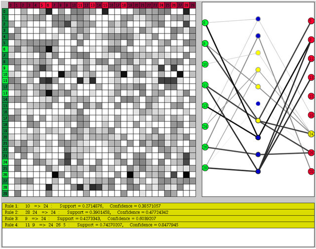
Figure 1. A screenshot of the SARV system. Note the matrix view of the entire set of association rules on the left, the graph view of the association rules related to a selection of items on the right, and a detailed view of the highlighted rules (related to RHS item 24, which is highlighted in yellow) on the bottom.
There have been numerous studies in the field of information visualization showing that good colour coding is an effective graphical device to reduce visual search time [32]. In SARV, colours are selected by following the guidance of the opponent process theory of colour [33]. According to this theory, there are three opponent channels: red vs. green, blue vs. yellow and black vs. white. The human visual processing system has a great ability to differentiate between colour hues within each of these channels. Based on this theory, red and green colours are used for encoding the RHS and LHS items, yellow and blue colours are used for showing highlighted and unhighlighted rules and items, and finally, grey-scale colours are used for coding different values of support.
Within the matrix view, colour darkness is used in order to distinguish between selected and unselected items within the LHS and RHS sets. Light green is used as a background colour of selected LHS items and dark green for unselected LHS items. Similarly, light red is used as a background colour of selected RHS items and dark red for unselected RHS items.
The matrix view allows users to visually identify rules based on the support measure. It employs colours between black and white for values between 1 and 0. The colour of each cell, corresponding to row r and column c represents the maximum support among all of the rules that have item r in the LHS and item c in the RHS. Although this colour coding does not make it possible to decode the specific quantitative support values, it does allow the user to perceive relative differences. Since determining the exact support values is not important in the overview window, the matrix view allow users to identify rules with higher support values (darker cells) and ignore rules with lower support values (lighter cells).
The primary drawback of this approach is that the number of items that can be shown simultaneously is limited by the screen space available for showing the matrix view. Although the screenshots and test data sets used in this paper do not have an exceedingly large number of items, the approach can scale by using a high-resolution display, supporting vertical and horizontal scrolling, or supporting zooming.
3.2.2. Interaction
Interaction is an important element in any visualization system. Allowing users to interact with system and to browse the association rules helps them to perceive different aspects of the rules and the relations between them. In order to avoid clutter in the graph view (which will be described next) and present interesting relations between LHS and RHS items, the matrix view allows users to filter items to focus on those that are of interest. As shown in Figure 2, users can select the LHS and RHS items they wish to investigate further by clicking on their associated labels. Selecting or unselecting items in this manner results in their appearance or disappearance from the graph view.
When users select a specific cell  in the matrix
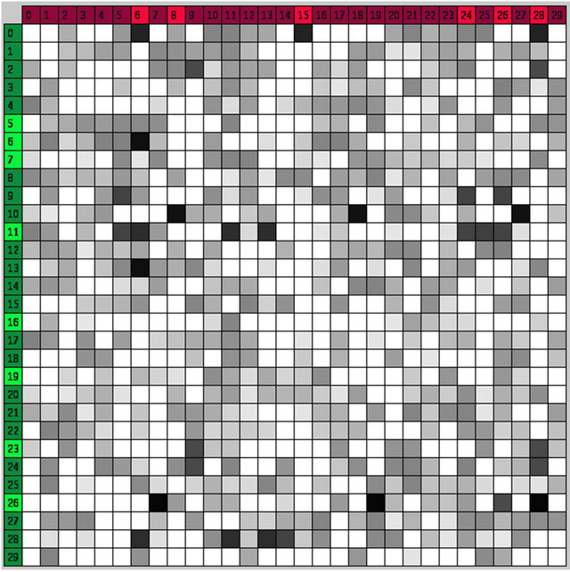
Figure 2. The matrix view shows the maximum support of the association rules (encoded as the grey-scale darkness) at the intersection of the LHS (left) and RHS (top) items.
view, the details of the rules that are related to that cell (i.e., have item c in their LHS and item r in their RHS) are shown in the detail view. For example, as illustrated in Figure 3, selecting the cell that corresponds to row 12 and column 21 results in showing three rules within the detail view. This information can then be used to determine whether the items associated with this cell are worthy of inclusion in the filter and further examination in the graph view.
3.3. Graph View
Once users select items from the LHS and RHS in the matrix view that they think may be important, they may wish to further understand the relationships among these rules. The goal of the graph view is to enable users to observe and inspect such relations, find the rules that are related to a specific item, and see the details of selected rules (items, relations, support and confidence).
3.3.1. Visual Encoding
As discussed previously, graphs can be used to represent association rules in a clear and concise manner. However, there is a limit on the number of relations and nodes that can reasonably be represented in a graph format; exceeding this limit results in visual clutter. In order to overcome this problem, a subset of the items may be selected in the matrix view. These items and the association rules that connect them are shown in the graph view.
In order to enable accurate decoding, a structured graph is employed to represent the subset of the association rules. Each green square on the left side of graph view represents an item that was selected from the LHS items of the matrix view. Similarly, each red square on the right side of the graph view represents an item that was selected from the RHS items of the matrix view. The blue circles in the middle represent the rules; the relations between the LHS and RHS items of the rules are represented with line segments that connect these items. Figure 4 shows a set of rules filtered from the matrix view, their items, and the graphical representation of the relations.
In this representation, the colour of the lines encodes the support of the rule (using the same grey-scale encoding that was used in the matrix view). In addition, the thickness of the lines encodes the confidence of the rules, where thicker lines represent higher confidence.
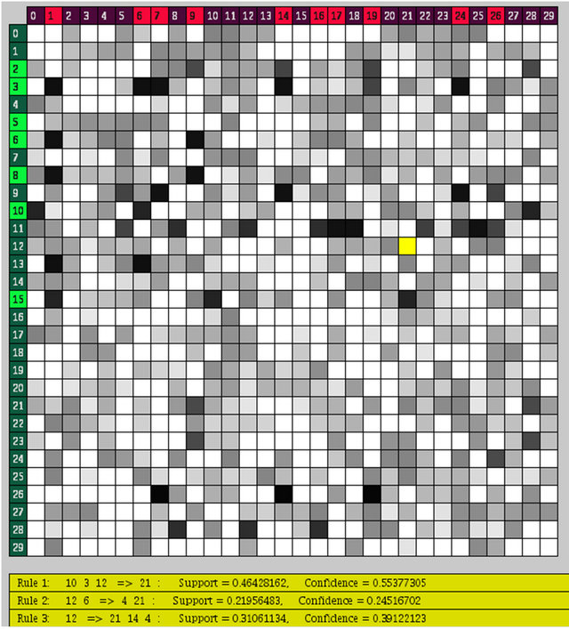
Figure 3. Selecting a cell in the matrix view shows all the rules that relate the corresponding LHS and RHS items in the detail view. Similarly, selecting specific rules from the graph view will show their full information in the detail view.
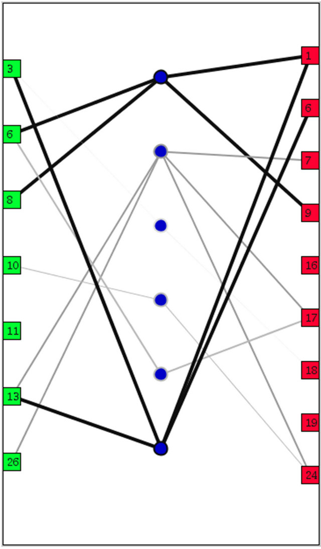
Figure 4. The graph view shows a subset of the association rules, connecting the LHS and RHS items through the rules. The edges in the graph encode the support (darkness of lines) and confidence (width of lines) of the rules.
As with the matrix view, there is a constraint on the number of LHS items, RHS items, and rules that can be reasonably displayed within the graph view. If too many are shown, the display will become congested and difficult to interpret. However, the intent of this view is not to show all possible rules for all items, but instead to show more details for a smaller subset of items of interest (selected via the matrix view), along with their associated rules. This view will scale to support more data by increasing the screen resolution and implementing scrolling or zooming operations.
3.3.2. Interaction
One of the important features of SARV is that it allows users to highlight rules related to specific items in the LHS or RHS. Once the user clicks an item in the LHS of the graph view, all rules that have this item in their LHS are highlighted in yellow. In the same way, when the user clicks an item in the RHS, all rules that have this item in their RHS are highlighted. Such highlighting mechanisms support the disambiguation of rules when there is a large degree of edge crossing within the graph view. In addition, the system shows the details of the highlighted rules in the detail view. Displaying the details of the rules helps users to further identify and understand specific information regarding these rules.
This highlighting feature not only helps users to find the relations between the rules, but also helps them to find the relations between items and rules. Furthermore, there is an additional highlighting feature that shows all related LHS and RHS items for a specific rule when the user clicks on the blue circles that represent the rules in the graph view. These two types of highlighting are shown in Figure 5.
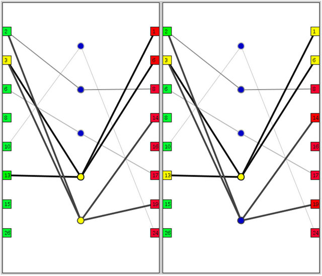
Figure 5. The highlighting feature in the graph view can be used to draw attention to the rules that are related to a specific item (e.g., item 3 in the LHS, as in the left screenshot). Alternately, specific rules can be highlighted that draw attention to all of the items that are connected through that rule (e.g.,  , as in the right screenshot). Yellow is used to show the highlighted elements.
3.4. Detail View
This view of the data shows the details of the rules that have been selected within the matrix view or graph view in a textual format (as shown at the bottom of Figure 3). As the users filter and evaluate association rules, they may wish to examine the specific details of the rules. This detail view shows the selected rules in a traditional textual format, including their precise values of support and confidence.
The detail view is visually encoded as a yellow region of the display. This colour is intentionally coordinated with the cell selection colour in the matrix view, and with the item and rule selection colour in the graph view. Whenever the user makes such a selection in these primary views, their selected element is highlighted in yellow, and the corresponding information is presented in the yellow detail view. This allows users to easily relate the information presented in the detail view back to its source location within the matrix and graph views. Since this detail view is primarily for information purposes, no other interaction is supported.
3.5. Scenarios of Use
The three distinct views of SARV (matrix view, graph view, and detail view) provide facilities for finding important association rules and the relations between them without loosing the “big picture” perspective of the entire set. Employing the combination of these views allows users to conduct different types of rule exploration. The two main activities that are usually undertaken in rule discovery processes are finding important association rules across the entire set of items, and finding important association rules related to a specified set of items. Here, we define important rules as those with strong support and confidence.
In order to find the important association rules using SARV, a user would first select the LHS and RHS items that correspond to the darker cells in the matrix view. These darker cells identify the rules that have higher support measures. The user could then inspect the specific association rules for a given cell by clicking on the cell, resulting in the display of the corresponding rules in the detail view. Selecting specific LHS and RHS items of interest in the matrix view would result in the loading of the rules that relate to these items into the graph view. Focusing on this selected subset of items and rules, the user could then find the important association rules by choosing the darker and thicker lines between the items in the graph view (representing the support and confidence for the rules, respectively). By selecting the central (blue) nodes in the graph view, the users could then view the specific details regarding the rules of interest.
If the user is instead interested in finding important association rules that are related to a specified set of items, they may seek the dark cells in the matrix view which correspond to the specific set of LHS and RHS items. For example, in order to find the important rules related to items i, j, and k, both the rows and columns corresponding to these items could be selected by the user. Doing so would show any relations between these items in the graph view. If the user is seeking other items that may also be related to this item set, they can visually scan the matrix view, seeking dark cells that are in the same rows or columns of the items of interest, inspecting the rules within these cells. They may then add any additional items they find in order to include their corresponding rules within the graph view. From there, the subset of rules can then be examined in detail, focusing on those that have dark and thick lines connecting the items to the rules.
In both of these scenarios, the user is empowered to discover interesting features within the potentially large set of association rules. The visual representation within the matrix view supports visual scanning activities and the identification of patterns within the rules. The graph view supports the interpretation of the relationships between the LHS and RHS items via the selected subset of rules. At any time, the user may inspect the details of the rules with a simple click operation in the matrix and graph views, showing the corresponding rules in the detail view.
4. Evaluation Methodology
SARV was designed to allow a large number of association rules to be presented simultaneously, allowing users to select interesting features and explore aspects of the association rules that are potentially useful. The goal was to create a system that would scale well, continuing to support the task of finding interesting and useful rules even as the total number of rules represented within the system grew. Although the system can also scale well as the number of items increases (by increasing the screen size of the matrix and graph views), our primary focus here is on the scalability with respect to the number of rules.
As an information visualization system, SARV allows users to visually identify and focus on the important association rules quickly and easily, even when there are a relatively large number of rules. While we may rationalize the various design choices made in the development of the system, since SARV is primarily a user interface to the underlying data, the true value of the approach can only be validated with user evaluations. The goal is to design a study that empirically measures both quantitative and qualitative data related to the use of the system, and ultimately to be able to make well-supported statements regarding its value [34].
4.1. Study Design
A user evaluation in a controlled laboratory setting was designed to study SARV. Two independent variables were defined and manipulated: the size of the data set (number of association rules), and the type of task to be performed. Five dependent variables were measured: time to task completion, error rates, confidence in the outcome of the task, ease of completing the task, and subjective measures regarding the system in general.
Three different data sets of varying sizes (50, 250, and 500 association rules) were made available to participants in the study. The goal in manipulating this independent variable was to determine whether the size of the underlying data set has an effect on the performance of the participants. Note that the number of items within these data sets remained constant (i.e., 30 items); what was manipulated was the number of association rules within the data set. In order to address potential learning effects, the order of exposure to the different data sets was varied using a 3 × 3 Latin Square, resulting in the assignment of participants to three different groups. As a result, the order in which the participants saw the data sets was eliminated as an independent variable.
Two different tasks were devised for participants to perform using SARV. The goal of the first task was for the participant to find the ten most significant association rules from the data set. The goal of the second task was for the participant to find the five most significant association rules that are related to a given set of three items. Here, we define significance of a rule as one that has a high support and confidence.
The tasks were provided as specific scenarios, asking the participants to consider themselves a knowledge manager within a company. The three different data sets contained the same number of items and the same number of association rules that satisfied the conditions of the tasks. The purpose in manipulating this independent variable was to determine if the type of task undertaken has an effect on the performance of the participants as the size of the data set is manipulated.
In order to simplify the study design, the participants performed the first task on all three data sets (in the order dictated by their group assignment), followed by the second task on all three data sets. The participants did not use the same data set for these two sequential tasks, which mitigated their ability to learn the answers to the second task by having just completed the first task on the same data set.
After gaining informed consent for participating in the study, a pre-study questionnaire was administered to each participant to measure their education level, prior experience with databases or data mining techniques, familiarity with association rules, and experience with data mining software. Although participants were prescreened to ensure they had sufficient prior knowledge about data mining techniques, a brief overview of association rules was provided in order to ensure a common baseline level of understanding of the domain.
As the participants performed each task, they were required to write down the association rules they found. The time they took to complete each task was measured. In addition, the investigator carefully observed the participants and took detailed notes regarding their use of the system. After each task, participants completed a short questionnaire regarding their confidence in the results obtained and the ease of completing the task.
After all tasks were completed, a post-study questionnaire was administered to measure subjective reactions to the use of the system in general. All participants in the study were financially compensated for their time.
4.2. Hypotheses
As a result of this study design, nine different hypotheses can be verified or refuted (four related to each of the two tasks, plus one related to the use of the system in general). In general, these hypotheses predict that the participants will be able to perform at a similar level, regardless of the increase in the number of association rules that need to be examined to complete the tasks.
H1: Participants will take a similar amount of time to find the ten most significant association rules, regardless of the size of the data set (50, 250, and 500 association rules).
H2: Participants will make a similar number of errors in finding the ten most significant association rules, regardless of the size of the data set (50, 250, and 500 association rules).
H3: Participants will report a similar level of confidence in finding the ten most significant association rules, regardless of the size of the data set (50, 250, and 500 association rules).
H4: Participants will report a similar level of ease in finding the ten most significant association rules, regardless of the size of the data set (50, 250, and 500 association rules).
H5: Participants will take a similar amount of time to find the five most significant association rules related to a given set of items, regardless of the size of the data set (50, 250, and 500 association rules).
H6: Participants will make a similar number of errors in finding the five most significant association rules related to a given set of items, regardless of the size of the data set (50, 250, and 500 association rules).
H7: Participants will report a similar level of confidence in finding the five most significant association rules related to a given set of items, regardless of the size of the data set (50, 250, and 500 association rules).
H8: Participants will report a similar level of ease in finding the five most significant association rules related to a given set of items, regardless of the size of the data set (50, 250, and 500 association rules).
H9: Participants will provide positive subjective responses to statements regarding the system in general.
4.3. Participants
A total of 12 participants were purposefully recruited from the graduate student population within our department. Participants were pre-screened to ensure they had taken at least one course in databases or data mining. The pre-study questionnaire verified a similar level of education and prior experience with association rules. As a result, we characterize the participants as knowledgeable users.
5. Evaluation Results
As a 3 × 2 (data set size × task type) within-subjects design, each participant performed a total of six tasks with the system. Due to the differences in the tasks (finding significant rules vs. finding significant rules associated with a given subset of items), this data cannot be combined, and direct comparisons between tasks are not informative. As such the results from each task are presented separately in the sections that follow. The primary analysis is to verify whether data set size has an impact on the participants’ performance. An analysis of the participants’ subjective reactions to using SARV after all the tasks were completed is provided at the end of this section.
5.1. Task 1: Finding Significant Association Rules
5.1.1. Time to Task Completion
The average time to task completion for each data set is illustrated in Figure 6. Using the time taken to complete the task with the 50 association rule data set as the baseline, on average there was a 1% reduction in the time to complete the task using the 250 association rule data set, and a 13% increase in time take to complete the task using the 500 association rule data set.
A pair-wise analysis of this data using ANOVA (see Table 1) found no statistical significance in the differences. As a result, we conclude that H1 (no differences in time to task completion regardless of data set size) is supported. That is, even though the number of association rules to examine increased by five and ten times, the time to find a set of ten significant rules did not change sufficiently to satisfy statistical significance.
5.1.2. Error Rates
Three different types of errors were identified based on the participants’ discovered association rules. These included participants identifying an association rule that did not meet the significance criteria, not being able to identify a sufficient number of association rules, and identifying duplicate association rules. The average number of each of these errors is illustrated in Figure 7.
Due to the extremely low error rate and the high degree of variability in the different types of errors, for the purposes of statistical verification, the errors were grouped together and a single ANOVA analysis was performed. The results from this analysis 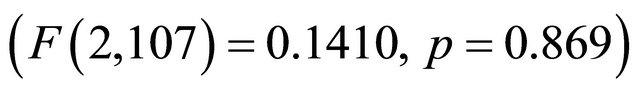 show that there is no statistical significance in the error rates as the number of association rules to be examined increases. As a result, we conclude that H2 is supported.
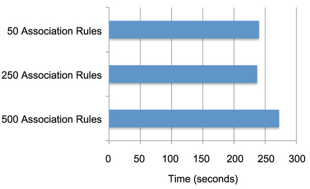
Figure 6. The average time to task completion for finding ten significant association rules using SARV (Task 1) for the data sets of three different sizes.
Table 1. Pair-wise comparison of time to task completion for Task 1 using ANOVA.
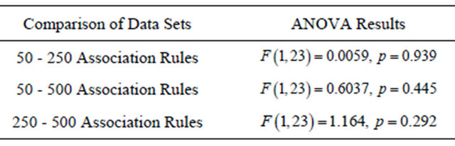
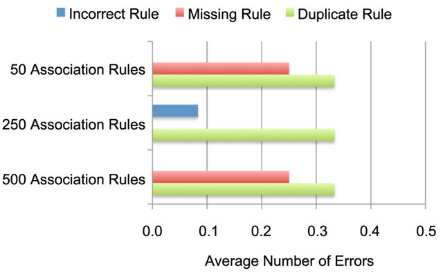
Figure 7. The average number of each of the different types of errors that were made during Task 1.
5.1.3. Confidence in Results
Confidence in the results of the task were measured after each task was completed, using a five-point Likert scale, ranging from very confident (5), through neutral (3), to very unconfident (1). Across all data sets, the scores ranged from three to five; the average scores are illustrated in Figure 8.
A pair-wise Wilcoxon-Mann-Whitney test was conducted on this subjective data to identify if there were any statistically significant differences as a result of completing the task with different sized data sets. The result of this analysis is reported in Table 2. Since no statistically significant differences were found, we conclude that H3 (participants will report a similar level of confidence regardless of the data set size) is supported. More specifically, even though the number of association rules to be examined increased across the data sets, the participants’ confidence in their results did not change.
5.1.4. Ease of Task Completion
As with the confidence measure, participants were asked to indicate the ease with which they were able to complete each task using a five-point Likert scale. The range of possible responses was from very simple (5), through neutral (3), to very difficult (1). The scores provided by the participants were similar to that of the confidence measure, ranging from three to five. The average scores are illustrated in Figure 9.
A pair-wise Wilcoxon-Mann-Whitney test was conducted to identify statistically significant differences between the data sets (see Table 3). As with the confidence
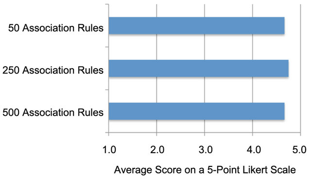
Figure 8. The average measure of confidence in the results of Task 1.
Table 2. Pair-wise comparison of the measure of confidence in the results of Task 1 using Wilcoxon-Mann-Whitney tests.
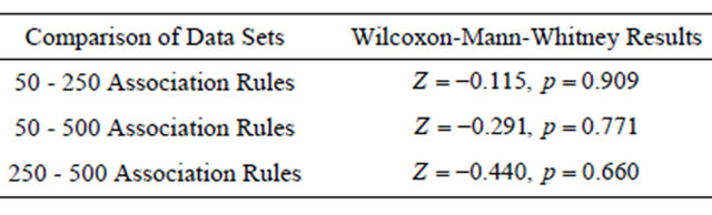
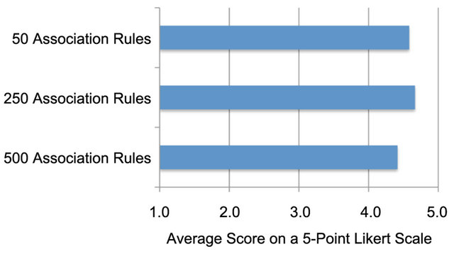
Figure 9. The average measure of the ease in completing Task 1.
Table 3. Pair-wise comparison of the ease of completing Task 1 using Wilcoxon-Mann-Whitney tests.
measure, no statistically significant differences were found due to the changing number of association rules to be examined, providing support for H4 (participants will report a similar level of ease in completing the task, regardless of the data set size).
5.1.5. Summary
The findings on Task 1 (finding the ten significant association rules) illustrate the key benefit of using SARV to examine the set of association rules. Even though the number of rules increased by factors of 5 and 10 over the smallest group of rules, the time to find the required set of rules, the error rates, the perceived confidence, and the perceived ease did not change. In particular, the ability to filter the association rules using the matrix view, and then examines the rules using the graph view and detailed view made the task equally as easy even as the number of rules available for examination increased.
5.2. Task 2: Finding Association Rules Related to a Given Item Set
5.2.1. Time to Task Completion
The average time to task completion for each data set is illustrated in Figure 10. Using the time taken to complete the task with the 50 association rule data set as the baseline, on average there was an 18% increase in the time to complete the task using the 250 association rule data set, and a 27% increase in time take to complete the task using the 500 association rule data set.
A pair-wise analysis of this data using ANOVA (see Table 4) found statistically significance differences be-
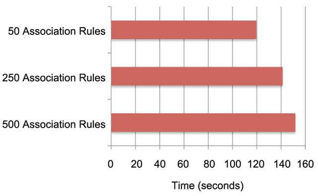
Figure 10. The average time to task completion for finding the five most significant association rules related to a given set of items using SARV (Task 2) for the data sets of three different sizes.
Table 4. Pair-wise comparison of time to task completion for Task 2 using ANOVA.
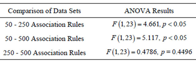
tween the 50 and 250 association rule data sets, and between the 50 and 500 association rule data sets. However, the difference between the 250 and 500 association rule data sets was not statistically significant. As a result, we conclude that H5 (no differences in time to task completion regardless of data set size) is not supported. That is, participants were able to perform the task faster when there were just 50 association rules to consider, when compared to having to consider 250 or 500 association rules.
The task required the participants to find five significant association rules from a set of 50, which were related to a given set of three items from the total of 30 items. As a result, the search space was already rather small, allowing the participants to be able to quickly complete the task without the need to take advantage of the key benefits of SARV. However, as the data sets became larger, the task became more difficult, requiring the participant to do more exploration within the data. As a result, they took more time to complete the task.
A positive note in this finding is that once the data sets became large enough to make the task difficult (i.e., data sets of size 250 and 500 association rules), there was no statistically significant difference in the participants time to task completion measurements. So, while we continue to hold that H5 is not supported, we believe that this is a result of the task being somewhat trivial when there are very few association rules to consider. As such, with a sufficiently large data set as the baseline, this hypothesis may become supported in future studies.
5.2.2. Error Rates
The average number of errors encountered during the completion of the task is illustrated in Figure 11. As with the previous task, due to the extremely low error rate and the high degree of variability in the types of errors, the errors were grouped together and a single ANOVA analysis was performed. The results from this analysis 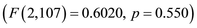 show that there is no statistical significance in the error rates between the different data sets. As a result, we conclude that H6 is supported. So even though the number of association rules to explore increased across the three data sets, there was virtually no difference in the ability of the participants to identify the most significant rules.
5.2.3. Confidence in Results
Confidence in the results of the task were measured using the same five-point Likert scale as in the first task. Across all data sets, the scores ranged from three to five; the average scores are illustrated in Figure 12.
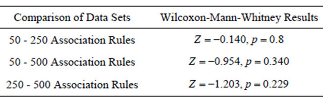
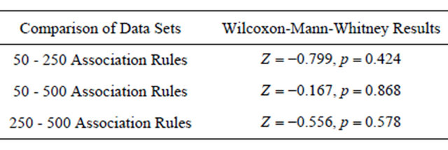
A pair-wise Wilcoxon-Mann-Whitney test was conducted on this subjective data to identify statistically significant differences as a result of completing the task with different data sets (Table 5). Since no statistically significant differences were found, we conclude that H7 (participants will report a similar level of confidence regardless of the data set size) is supported.
5.2.4. Ease of Task Completion
A similar five-point Likert scale was used to measure participants’ impressions of the ease of completing the task. The scores provided by the participants were similar to that of the confidence measure, ranging from three to five. The average scores are illustrated in Figure 13.
A pair-wise Wilcoxon-Mann-Whitney test was conducted to identify statistically significant differences between the data sets (see Table 6). No statistically sig-

Figure 11. The average number of each of the different types of errors that were made during Task 2.

Figure 12. The average measure of confidence in the results of Task 2.
Table 5. Pair-wise comparison of the measure of confidence in the results of Task 2 using Wilcoxon-Mann-Whitney tests.
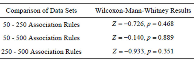
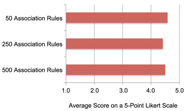
Figure 13. The average measure of the ease in completing Task 2.
Table 6. Pair-wise comparison of the ease of completing Task 2 using Wilcoxon-Mann-Whitney tests.
nificant differences were found, providing support for H8 (participants experiencing a similar level of ease in completing the task, regardless of the data set size).
5.2.5. Summary
Similar to Task 1, the findings on Task 2 (finding the five most significant association rules related to a subset of items) highlight the benefits of using SARV to explore among the association rules. Even as the number of association rules varied by a factor of ten, all of the measures except for the time to task completion remained essentially unchanged. When there were only 50 total association rules, participants were able to find the five most significant that referenced the small subset of items much quicker than when the number of rules got larger. Even so, the error rates, perceived confidence, and perceived ease were consistent across all sizes of the data.
5.3. Subjective Reactions
After completing all of the tasks with all of the data sets, participants were asked to rank their subjective agreement to a number of statements using a five-point Likert scale. The response options ranged from strongly agree, through neutral, to strongly disagree. Figure 14 illustrates the responses for five particularly useful measures. In nearly all cases, participants reported either agreeing or strongly agreeing with the statements.
Since the study design did not provide a baseline against which these responses can be compared, conducting a statistical analysis of the data is not meaningful. However, we can conclude that there are substantial positive reactions to the learnability, visual encodings, ease of use, and utility of SARV, which support H9 (participants will provide positive subjective reactions to the system in general).
6. Conclusions
In this paper we proposed a new technique for the visualization of association rules. SARV presents the association rules in three synchronized views: the matrix view providing an overview of the rules, the graph view illustrating relationships and further details on a subset of rules, and the detail view showing the complete information of selected rules and/or items. The system was designed with the purpose of scaling well as the number of association rules becomes large, while avoiding the problems of occlusion and visual clutter.
SARV was designed to follow Shneiderman’s visual information seeking matra of “over view first, zoom and filter, then details on demand”. An overview of the entire set of the rules is provided in the matrix view. The user may use this to filter the rules based on LHS and RHS items of interest, populating the graph view with the corresponding rules. This subset of the rules can be visually inspected further, allowing the user to gain a better understanding of the relationships that the rules represent. At any point, the specific details of the rules can be accessed and evaluated.
A user study was performed to verify the scalability of SARV with respect to the number of rules being repre-
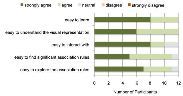
Figure 14. Frequency of subjective reaction response, as measured at the end of the study.
sented. The results of this study showed that with only one minor exception, participants were able to find a set of the most significant rules, as well as the significant rules related to a given set of items, in approximately the same time with the same error rate for data sets that contained small (50), medium (250) and large (500) numbers of rules. In addition, subjective measures showed that the participants’ perceptions of confidence and ease in completing the task did not differ with the size of the data set. Subjective responses to the system in general were also very positive. These results show the value of the visualization and interactive filtering features of SARV.
For future work, we plan to add features such as multiselection in order to allow users to compare the rules, the visual representation of other interestingness measures, and support for more complex association rules such as dynamic association rules, quantitative association rules, and weighted association rules. In addition, we plan to perform additional user studies to measure the scalability of the approach as the number of items within the dataset grows.
REFERENCES
- P. Buono and M. F. Costabile, “Visualizing Association Rules in a Framework for Visual Data Mining,” In: M. Hemmje, C. Niederée and T. Risse, Eds., From Integrated Publication and Information Systems to Virtual Information and Knowledge Environments, Springer Berlin Heidelberg, Berlin, 2005, pp. 221-231. doi:10.1007/978-3-540-31842-2_22
- B. Shneiderman, “The Eyes Have It: A Task by Data Type Taxonomy for Information Visualizations,” Proceedings of the IEEE Symposium on Visual Languages, Boulder, 3-6 September 1996, pp. 336-343. doi:10.1109/VL.1996.545307
- O. Couturier, J. Rouillard and V. Chevrin, “An Interactive Approach to Display Large Sets of Association Rules,” Proceedings of Symposium on Human Interface and the Management of Information, Methods, Techniques and Tools in Information Design, Beijing, 22-27 July 2007, pp. 258-267.
- O. Couturier, T. Hamrouni, S. B. Yahia and E. M. Nguifo, “A Scalable Association Rule Visualization towards Displaying Large Amounts of Knowledge,” Proceedings of the International Conference on Information Visualization, Zuric, 4-6 July 2007, pp. 657-663. doi:10.1109/IV.2007.16
- C. H. Yamamoto, M. C. Oliveira and S. O. Rezende, “Including the User in the Knowledge Discovery Loop: Interactive Itemset-Driven Rule Extraction,” Proceedings of the ACM Symposium on Applied Computing, Fortaleza, 16-20 March 2008, pp. 1212-1217.
- R. Agrawal and R. Srikant, “Fast Algorithms for Mining Association Rules,” Proceedings of the International Conference on Very Large Databases, Santiago de Chile, 12-15 September 1994, pp. 125-131.
- L. Geng and H. J. Hamilton, “Interestingness Measures for Data Mining: A Survey,” ACM Computing Surveys, Vol. 38, No. 3, 2006, pp. 1-32. doi:10.1145/1132960.1132963
- R. J. Hilderman and H. J. Hamilton, “Measuring the Interestingness of Discovered Knowledge: A Principled Approach,” Intelligent Data Analysis, Vol. 7, No. 4, 2003, pp. 347-382.
- L. Berti-Équille, “Data Quality Awareness: A Case Study for Cost Optimal Association Rule Mining,” Knowledge and Information Systems, Vol. 11, No. 2, 2007, pp. 191- 215. doi:10.1007/s10115-006-0006-x
- B. Shen, M. Yao, Z. Wu and Y. Gao, “Mining Dynamic Association Rules with Comments,” Knowledge and Information Systems, Vol. 23, No. 1, 2010, pp. 73-98. doi:10.1007/s10115-009-0207-1
- Y. Ke, J. Cheng and W. Ng, “An Information-Theoretic Approach to Quantitative Association Rule Mining,” Knowledge and Information Systems, Vol. 16, No. 2, 2008, pp. 213-244. doi:10.1007/s10115-007-0104-4
- W. Wang, J. Yang and P. Yu, “WAR: Weighted Association Rules for Item Intensities,” Knowledge and Information Systems, Vol. 6, No. 2, 2004, pp. 203-229.
- A. Ceglar, J. Roddick, P. Calder and C. Rainsford, “Visualising Hierarchical Associations,” Knowledge and Information Systems, Vol. 8, No. 3, 2005, pp. 257-275. doi:10.1007/s10115-003-0139-0
- G. A. Miller, “The Magical Number 7 Plus or Minus 2: Some Limits on Our Capacity for Processing Information,” Psychological Review, Vol. 63, No. 1, 1956, pp. 81-97. doi:10.1037/h0043158
- R. Spence, “Information Visualization: Design for Interaction,” 2nd Edition, Prentice Hall, Upper Saddle River, 2007.
- C. Ware, “Information Visualization: Perception for Design,” 2nd Edition, Morgan Kaufmann, Burlington, 2004.
- M. Ward, G. Grinstein and D. Keim, “Interactive Data Visualization: Foundations, Techniques, and Applications,” A. K. Peters, Natick, 2010.
- S. K. Card, J. D. Mackinlay and B. Shneiderman, “Readings in Information Visualization, Morgan Kaufmann, Burlington, 1999.
- B. Zhu and H. Chen, “Information Visualization,” Annual Review of Information Science and Technology, Vol. 39, No. 1, 2005, pp. 139-177. doi:10.1002/aris.1440390111
- E. Tufte, “The Visual Display of Quantitative Information,” 2nd Edition, Graphics Press, Cheshire, 2001.
- K. Techapichetvanich and A. Datta, “VisAR: A New Technique for Visualizing Mined Association Rules,” Proceedings of the International Conference on Advanced Data Mining and Applications, Wuhan, 22-24 July 2005, pp. 88-95.
- C. Romero, J. M. Luna, J. R. Romero and S. Ventura, “RM-Tool: A Framework for Discovering and Evaluating Association Rules,” Advances in Engineering Software, Vol. 42, No. 8, 2011, pp. 566-576. doi:10.1016/j.advengsoft.2011.04.005
- A. Inselberg and B. Dimsdale, “Parallel Coordinates: A Tool for Visualizing Multi-Dimensional Geometry,” Proceedings of the IEEE Conference on Visualization, 1990, pp. 361-378. doi:10.1109/VISUAL.1990.146402
- M. Hahsler, S. Chelluboina, K. Hornik and C. Buchta, “The Arules R-Package Ecosystem: Analyzing Interesting Patterns from Large Transaction Data Sets,” Journal of Machine Learning Research, Vol. 12, No. 1, 2011, pp. 2021-2025.
- L. Yang, “Visual Exploration of Frequent Itemsets and Association Rules,” In: S. J. Simoff, M. H. Böhlen and A. Mazeika, Eds., Visual Data Mining: Theory, Techniques and Tools for Visual Analytics, Springer Berlin Heidelberg, Berlin, 2008, pp. 60-75. doi:10.1007/978-3-540-71080-6_5
- L. Yang, “Pruning and Visualizing Generalized Association Rules in Parallel Coordinates,” IEEE Transactions on Knowledge and Data Engineering, Vol. 17, No. 1, 2005, pp. 60-70. doi:10.1109/TKDE.2005.14
- W. S. Cleveland and R. McGill, “Graphical Perception: The Visual Decoding of Quantitative Information on Statistical Graphs,” Journal of the Royal Statistical Society, Vol. 150, No. 1, 1987, pp. 192-229. doi:10.2307/2981473
- H. H. Ong, K. L. Ong, W. K. Ng and E. P. Lim, “Crystal Clear: Active Visualization of Association Rules,” Proceedings of the International Workshop on Active Mining, Maebashi City, 9 December 2002, pp. 123-132.
- H. Hofmann, A. P. Siebes and A. F. Wilhelm, “Visualizing association rules with Interactive Mosaic Plots,” Proceedings of the ACM SIGKDD International Conference on Knowledge Discovery and Data Mining, Boston, 20-23 August 2000, pp. 227- 235.
- J. Blanchard, B. Pinaud, P. Kuntz and F. Guillet, “A 2D- 3D Visualization Support for Human-Centered Rule Mining,” Computers & Graphics, Vol. 31, No. 1, 2007, pp. 350-360. doi:10.1016/j.cag.2007.01.026
- A. Noraziah, Z. Abdullah, T. Herawan and M. M. Deris, “WLAR-Viz: Weighted Least Association Rules Visualization,” Proceedings of Information Computing and Applications, Chengde, 14-16 September 2012, pp. 592-599.
- S. Chakravarthy and H. Zhang, “Visualization of Association Rules over Relational DBMSs,” Proceedings of the ACM Symposium on Applied Computing, Melbourne, 9-12 March 2003, pp. 922-926.
- E. Hering, “Outlines of a Theory of the Light Sense (Translated by L. M. Hurvich and D. Jameson),” Harvard University Press, Harvard, 1964. doi:10.1016/0001-6918(64)90135-0
- S. Carpendale, “Evaluating Information Visualizations,” In: A. Kerren, J. T. Stasko, J.-D. Fekete and C. North, Eds., Information Visualization: Human-Centered Issues and Perspectives, Springer Berlin Heidelberg, Berlin, 2008, pp. 19-45. doi:10.1007/978-3-540-70956-5_2