International Journal of Intelligence Science
Vol.2 No.4A(2012), Article ID:24181,8 pages DOI:10.4236/ijis.2012.224018
Learn More about Your Data: A Symbolic Regression Knowledge Representation Framework
Karlsruhe University of Applied Sciences, Karlsruhe, Germany
Email: Ingo.Schwab@hs-karlsruhe.de, Norbert.Link@hs-karlsruhe.de
Received June 30, 2012; revised August 8, 2012; accepted August 19, 2012
Keywords: Classification; Symbolic Regression; Knowledge Management; Data Mining; Pattern Recognition
ABSTRACT
In this paper, we propose a flexible knowledge representation framework which utilizes Symbolic Regression to learn and mathematical expressions to represent the knowledge to be captured from data. In this approach, learning algorithms are used to generate new insights which can be added to domain knowledge bases supporting again symbolic regression. This is used for the generalization of the well-known regression analysis to fulfill supervised classification. The approach aims to produce a learning model which best separates the class members of a labeled training set. The class boundaries are given by a separation surface which is represented by the level set of a model function. The separation boundary is defined by the respective equation. In our symbolic approach, the learned knowledge model is represented by mathematical formulas and it is composed of an optimum set of expressions of a given superset. We show that this property gives human experts options to gain additional insights into the application domain. Furthermore, the representation in terms of mathematical formulas (e.g., the analytical model and its first and second derivative) adds additional value to the classifier and enables to answer questions, which sub-symbolic classifier approaches cannot. The symbolic representation of the models enables an interpretation by human experts. Existing and previously known expert knowledge can be added to the developed knowledge representation framework or it can be used as constraints. Additionally, the knowledge acquisition framework can be repeated several times. In each step, new insights from the search process can be added to the knowledge base to improve the overall performance of the proposed learning algorithms.
1. Introduction
Supervised classification algorithms aim to assign a class label for each input example. We have given a training dataset of the form , where
  is the ith example and
  is the ith class label in a binary classification task.
  can be composed of any number type and
  can be any value of a bi-valued set as well. This means that we restrict our considerations to two-class problems. This imposes no restriction since multi-class problems can be represented by combination of two-class problems. A model
  is learned, so that it is
  for new unseen examples. In fact, it is an optimization task and the learning process is mainly data driven. It results in an adaptation of the model that reproduces the data with as few errors as possible. Several algorithms have been proposed to solve this task and the result of the learning process is an internal knowledge model
 .
.
There are basically two ways to represent the knowledge of model . The first approach includes algorithms like Naïve Bayes Classifiers, Hidden Markov Models or Belief density functions and priors [1]. The main idea is to represent the knowledge as a probability distribution. The classification boundary is the intersecttion of the posterior probabilities of the classes in Bayes decision theory.
The other approach for representing the knowledge is to determine a surface in the feature space which separates the samples of the different classes of the training data as well as possible. The decision surface is represented by parameterized functions which can be the sum of weighted base functions of one dedicated function class. Examples include the logistic functions and radial basis functions, which can be used in Neural Networks and Support Vector Machines [1].
It is important to point out that the base functions are closely linked to the used classifiers. Our approach further refines this idea (Sections 2 and 3). Again, the decision surface is determined by a level surface of a model function. However, in this case, the function is composed of an arbitrary (but predefined) set of mathematical symbols, forming a valid expression of a parameterized function. This approach allows the human users of the system to control the structure and complexity of the solutions.
Following this idea, we try to find solutions which are as short and understandable as possible. Additionally, the selected solutions should model the dataset as well as possible. Clearly, these are mostly opposing requirements and nature of multi-objective decision making. Therefore, we select all good compromises of the pareto front [2] and sort them by complexity. This approach extends the concept presented in [3] and helps human experts to choose the best compromise. In standard classification approaches (e.g., Neural Networks), where the structure of the base functions is predefined, structural complexity is always required to reflect highly structured data. In most nontrivial applications the learned models are not understandable to the human expert and the represented knowledge cannot therefore be refined and reused for other purposes [4].
There are many different ways to further subdivide this class of learning algorithms (e.g., greedy and lazy, inductive and deductive [5] variants). In this paper, we focus on the symbolic and sub-symbolic knowledge representation paradigm (see [4,6] for more details) and its consequences for the reusability of the model  and the inherently learned knowledge. This subdivision separates the approaches with symbolic representations in which the knowledge of the model
  is characterized by explicit symbols, from sub-symbolic representations which are associated with parameter values. One of the main disadvantages of sub-symbolic classifiers (e.g., Neural Network or Support Vector Machine) is that the class of classifiers includes the properties of a black box and the learned model cannot be easily interpreted or reformulated.
The main advantages of our approach (see Subsection 3.2) are determined by the nature of mathematical formulas. They can be interpreted by humans and there are many rules to reformulate, simplify and derive additional information from. The additional information can be used for stability tests in order to build robust classifiers. In fact, reformulating mathematical formulas is one of the most important areas of mathematics. For the black box character of the sub-symbolic learning algorithms such rules simply do not exist.
The remaining part of this paper is arranged as follows. In Section 2, necessary information and the used Symbolic Regression algorithm are presented. Section 3 summarizes our approach and shows how to generalize the regression task for classification. Furthermore, the main advantages of the approach are briefly discussed. Section 4 explains some of our experiments and Section 5 concludes with final remarks.
2. Background and Related Work
2.1. Symbolic vs. Subsymbolic Representation
As Smolensky [6] noted, the term sub-symbolic paradigm is intended to suggest symbolic representations that are built out of many smaller constituents: “Entities that are typically represented in the symbolic paradigm by symbols are typically represented in the sub-symbolic paradigm by a large number of sub-symbols”.
The debate over symbolic versus sub-symbolic representations of human cognition is this: Does the human cognitive system use symbols as a representation of knowledge? Or does it process knowledge in a distributed representation in a complex and meaningful way? e.g., in Neural Networks the knowledge is represented in the parameters of the model. It is not possible to determine the exact position of the knowledge and the observed system variable of the data set.
From this point of view, the syntactic role of sub-symbols can be described as the sub-symbols participate in numerical computation. In contrast, a single discrete operation in the symbolic paradigm is often achieved in the sub-symbolic paradigm by a large number of much finergrained operations. One well known problem with subsymbolic networks which have undergone training is that they are extremely difficult to interpret and analyze. In [4], it is argued that it is the inexplicable nature of mature networks. Partially, it is due to the fact that sub-symbolic knowledge representations cannot be interpreted by humans and that they are black box knowledge representations.
2.2. Pareto Front
In this subsection we discuss the pareto front or pareto set in multi-objective decision making [2]. This area of research has a strong impact on machine learning and data mining algorithms.
Many problems in the design of complex systems are formulated as optimization problems, where design choices are encoded as valuations of decision variables and the relative merits of each choice are expressed via a utility or cost function over the decision variables.
In most real-life optimization situations, however, the cost function is multidimensional. For example, a car can be evaluated according to its cost, power, fuel consumption, passenger room, speed, and a configuration s which is better than s* according to one criteria and can be worse according to another.
Let us consider an optimization problem with n objective functions [7]. The n objectives form a space called objective space . A design variable is represented by a vector in a decision space
 . The set
  of the elements satisfying all the constraints is called a feasible set or feasible space. For each
  there exists a point in
  corresponding to mapping
 .
.
Hence, the feasible objective space , is the image of
 , i.e.
 . A generic form of any multi-objective optimization is given by
 (1)
(1)
Definition II.1 (Pareto Optimality) Vector  is called a pareto solution to problem (1) iff
  such that,
 and
and  :
: .
.
Consequently, there is no unique optimal solution but rather a set of efficient solutions, also known as pareto solutions, characterized by the fact that their cost cannot be improved in one dimension without being worsened in another.
In machine learning algorithms, the competing optimization criteria  and
and  are the prediction accuracy and the size and complexity of the learning model.
The set of all pareto solutions, the pareto front, represents the problem trade-offs, and being able to sample this set in a representative manner is a very useful aid in decision making.
Vector  is called a local pareto solution if Definition II.1 holds in
  -vicinity of
 . If
. If  is a pareto solution it is said that
  is not dominated by any other feasible solutions.
In our approach, the solutions are ordered by complexity. Through the symbolic representation the human expert is able to interpret the solutions of the pareto front (Section 4.3).
2.3. Classical Regression Analysis and Symbolic Regression
Regression analysis [8] is one of the basic tools of scientific investigation. It enables identification of functional relationships between independent and dependent variables. The general task of regression analysis is defined as identification of a functional relationship between the independent variables x = [alt x1, x2, …, xn] and dependent variables y = [alt y1, y2, ..., ym], where n is the number of independent variables in each observation and m is the number of dependent variables.
The task is often reduced from an identification of an arbitrary functional relationship f to an identification of the parameter values of a predefined (e.g., linear) function. That means that the structure of the function is predefined by a human expert and only the free parameters are adjusted. From this point of view Symbolic Regression goes much further.
Like other statistical and machine learning regression techniques Symbolic Regression also tries to fit observed experimental data. But unlike the well-known regression techniques in statistics and machine learning, Symbolic Regression is used to identify an analytical mathematical description and it has more degrees of freedom in building it. A set of predefined (basic) operators is defined (e.g., add, multiply, sin, cos) and the algorithm is mostly free in concatenating them. In contrast to the classical regression approaches which optimize the parameters of a predefined structure, here also the structure of the function is free and the algorithm both optimizes the parameters and the structure of the base functions.
There are different ways to represent the solutions in Symbolic Regression. For example, informal and formal grammars have been used in Genetic Programming to enhance the representation and the efficiency of a number of applications including Symbolic Regression [9].
Since Symbolic Regression operates on discrete representations of mathematical formulas, non-standard optimization methods are needed to fit the data. The main idea of the algorithm is to focus the search on promising areas of the target space while abandoning unpromising solutions (see [5,10] for more details). In order to achieve this, the Symbolic Regression algorithm uses the main mechanisms of Genetic and Evolutionary Algorithms. In particular, these are mutation, crossover and selection [10] which are applied to an algebraic mathematical representation.
The representation is encoded in a tree [10] (Figure 1). Both the parameters and the form of the equation are subject to search in the target space of all possible mathematical expressions of the tree. The operations are nodes in the tree (Figure 1 represents the formula 6x + 2) and can be mathematical operations such as additions (add), multiplications (mul), abs, exp and others. The terminal values of the tree consist of the function’s input variables and real numbers. The input variables are replaced by the values of the training dataset.
In Symbolic Regression, many initially random symbolic equations compete to model experimental data in the most promising way. Promising are those solutions which are a good compromise between correct prediction quality of the observed and experimental data and the length of the computed mathematical formula.
Mutation in a symbolic expression can change the mathematical type of formula in different ways. For example, a div is changed to an add, the arguments of an operation are replaced (e.g., change 2*x to 3*x), an operation is deleted (e.g., change 2*x + 1 to 2*x), or an operation is added (e.g., change 2*x to 2*x + 1).
The fitness objective in Symbolic Regression, like in other machine learning and data mining mechanisms, is to minimize the regression error on the training set. After
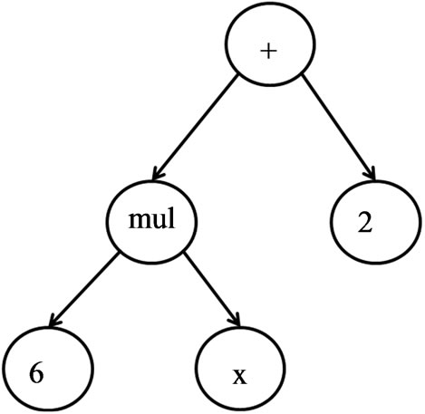
Figure 1. Tree representation of the equation 6x + 2.
an equation reaches a desired level of accuracy, the algorithm returns the best equation or a set of good solutions (the pareto front). In many cases the solution reflects the underlying principles of the observed system.
3. Proposed Method
This section explains our knowledge acquisition workflow (Figure 2). The core of the workflow is structured in 4 steps.
1) The human expert defines the set of base functions. The functions should be adapted to the domain problem. For example, many geometrical problems are much easier to solve with trigonometric base functions.
2) The second step in the workflow is the main optimization process ([11], Section 2.3 and 3.1 of this paper for more details) which adopts the model to the experimental data. Symbolic Regression is used to solve this task. The step is repeated until the model has the desired prediction quality. It should be noted, however, that other optimization algorithms which can handle discrete black box optimization can be used for this task.
3) A human expert can interpret and reformulate the solutions of the pareto front (Section 4.3).
4) The knowledge can be refined automatically or by human users. Afterwards it can be reused and transferred to other domains. Additionally, the new domain knowledge can be used as a feedback loop to further optimize and guide the learning process.
Figure 3 represents the knowledge flow between the different knowledge bases and the learning algorithms. It adds a complementary point of view to Figure 2.
In Figure 3, the core of the Knowledge Acquisition Flow System (Figure 2) is highlighted by the grey circle. System observations form experimental data which is the training data of the learning process. Based on this data the knowledge acquisition workflow is started. Again, Symbolic Regression is used to optimize the learning model (Section 2.3) in order to reproduce the experimental data. When the desired prediction quality is reached, the model (respectively the pareto front) is analyzed and reformulated. This step can be done automatically or by a human expert. The additional knowledge is
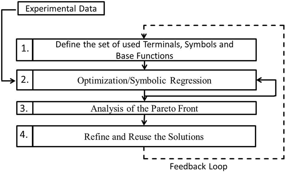
Figure 2. The knowledge acquisition workflow.
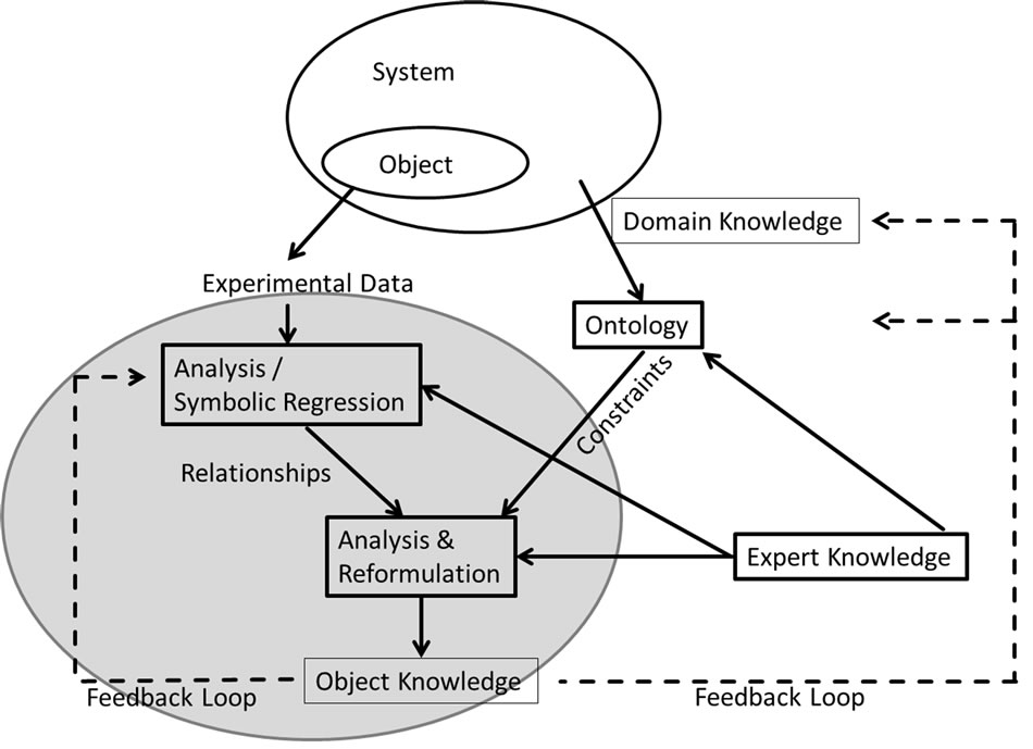
Figure 3. The knowledge flow.
stored in an object knowledge database. This information forms an input to further improve the optimization step of the Symbolic Regression.
In addition, the object knowledge can be used to improve the domain knowledge. In the domain knowledge database existing knowledge is stored. Additionally, this knowledge can also be stored in an ontology. An example is presented in Subsection 4.3 (e.g., human experts know that the age of the patients or the number of axillary nodes cannot be negative). These constraints help the search to further improve the quality of the model. Additionally, it helps by reformulation of the computed models.
Even though the whole knowledge flow can be executed automatically the quality of the learned models will be higher if the search is guided by the additional knowledge of a human user.
3.1. From Regression to Classification
So far the regression task was described in this paper. To be able to use the system for a classification task several additions have to be undertaken. The necessary modifications are described in this subsection.
First, an activation function is defined. In our approach it is a step function which is defined as
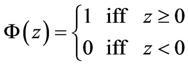 .
.
We have given a training set of N feature vectors 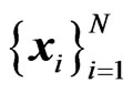 and assigned class labels
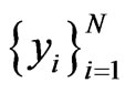 ,
, . The main challenge and computer time consuming task is to find a function f which transforms the input space in the way that
  with as few errors as possible. In other words, a function
  is sought with
  separating the areas of the feature space, where the vectors of the different classes are located. The zero-crossing
  therefore defines the decision surface. So far, the approach is Perceptron-like [12]. Instead of replacing the step-functions by continuous and differentiable base functions to allow cost function optimization, Symbolic Regression is used to optimize the cost function
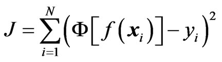 and therefore to find
 .
.
The main advantage of this approach is due to the fact that complexity and interpretability of the solution can be controlled by the user by the set of allowed operations and by selecting the appropriate complexity by means of the pareto front. Further approach advantages (see the next subsection) are consequences of this property.
3.2. Advantages
In this subsection we summarize the additional advantages of the proposed approach [13,14]. It should be noted that all mathematical reformulations of the classifier do not change its behavior in classification:
• Select Variables and Metavariables: Often more variables are available in the observed system behavior than required. Selecting the important critical variables is a dimension reduction problem and helps to focus the search. For the algorithm it is easier to concentrate the search on the underlying system principles rather than system noise. Additionally, Symbolic Regression is useful for identifying meta-variables. In [15] an approach is presented which collects the functional terms of the pareto front of several repeated Symbolic Regression runs. On this set of terms a frequency analysis is conducted. The assumption of this approach is that the more frequent terms form a kind of meta-variables and help to explain the system behavior. Additionally the meta-variables identified via Symbolic Regression can enable model linearization which is preferable from a robustness perspective.
• Modeling: Many techniques are available for model building. These include fitting simple mathematical models (e.g., polynomials) as well as nonlinear datadriven techniques. This class of algorithms includes Support Vector Machines and Neural Networks. Generally, it can be said that the class of sub-symbolic classifiers is able to generate more accurate classifiers. The main advantage of Symbolic Regression is that it generates more understandable models. To be understandable to human experts our approach tries to find solutions which are as simple as possible. The pareto front [2] sorts the solutions by complexity and prediction quality.
• Analyze and Validate Models: Any model based on empirical data should be viewed with suspicion. Until it proves its validity the possibility of over-fitting must be explored as well as the reasonableness of the results. Additionally, most of the times the behavior of the model outside the domain of the data sample is un-known. Data partitioning and data cleaning can help in finding a robust model. However, the symbolic representation of the learned models enables human experts to interpret the model and its behavior. e.g., the decision area can be calculated analytically. Most of the known sub-symbolic learning algorithms are not able to answer these questions.
• Add Additional Domain Knowledge to the Model: It is difficult to add additional human expert domain knowledge (e.g., from textbooks) to sub-symbolic knowledge representations. One possible way is to add it in form of regularization constraints. From this point of view Symbolic Regression is more flexible. e.g., the domain knowledge can be the starting point of the initialization of the Symbolic Regression search process.
• Analytically Calculate the Derivative of the Learned Model: One of the main advantages is that the proposed approach enables us to calculate the derivatives of the classifier. It should be mentioned, that this can also be done for most sub-symbolic knowledge representations. But in this case the derivative is also sub-symbolic. In our approach the derivatives are in the general case symbolic and can be interpreted by humans.
• One scenario for application could be in engineering technologies or medical systems. For example it could be the task to learn when a work-piece is damaged or when there is a risk of a certain illness. The general learning approaches enable only the class prediction (e.g., defect or no defect). With the first derivative, which can be analytically calculated by our approach we can also say which attributes of the classifier should be changed (and in which direction) in order to leave the undesired class as soon as possible. Additionally, the numerically or symbolically differentiated model can be used to understand the sensitivity to parameter changes. This can be useful in applications which require a robust design.
• Select and Combine Models: The best model may not be the most accurate depending upon the definitions of classification accuracy. For example, understandable models with sufficient exact prediction accuracy may be preferred. This idea includes a concept, that more complex models have a tendency to model noise of the observed system. Combining models, e.g., stacking or boosting [16] can result in improved performance as well as an indication of operation in unknown regions of parameter space.
• Exploit Models: In an industrial setting, the modeling effort is not a success unless the models are being exploited either by providing system insight, enabling optimization or deployed in an operational system. In addition, it is beneficial if the model knowledge can be reused in other domains. A symbolic knowledge re-presentation enables us to extract or validate and subsequently transfer the knowledge to other domains.
4. Experiments and Results
This section discusses and demonstrates some of the conducted experiments. First we show two experiments based on artificial datasets while the third described experiment is based on a real-word dataset.
4.1. First Experiment
Figure 4 shows the data of a two class learning tasks in a two-dimensional plot. The first class is represented by the circles and the second by the triangles. The zerocrossing  decision boundary of the different classes of formula 2 (calculated by our Symbolic Regression algorithm) is displayed in Figures 4 and 5 by the parabola.
In order to find interpretable formulas we restricted the search on using add, sub, mul and all real numbers as operators.
 (2)
(2)
As discussed in Section 3, it is easy for a human expert to interpret this solution. It is a representation of an ellipse. With this knowledge the user can conclude much more about the domain. The additional knowledge includes conclusions about the decision area. Based on their high complexity, black box machine learning algorithms usually give no additional insight into its behavior.
As a result of the interpretable analytical solution (Formula 2) we know that there is only one decision boundary (the zero-crossing). This knowledge is essential for some domains (application scenarios can include medical or other critical domains) which require robust classifiers. This robustness includes predictable behaviour of un-
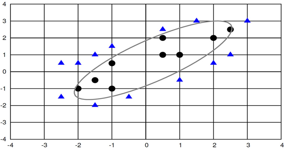
Figure 4. First dataset.
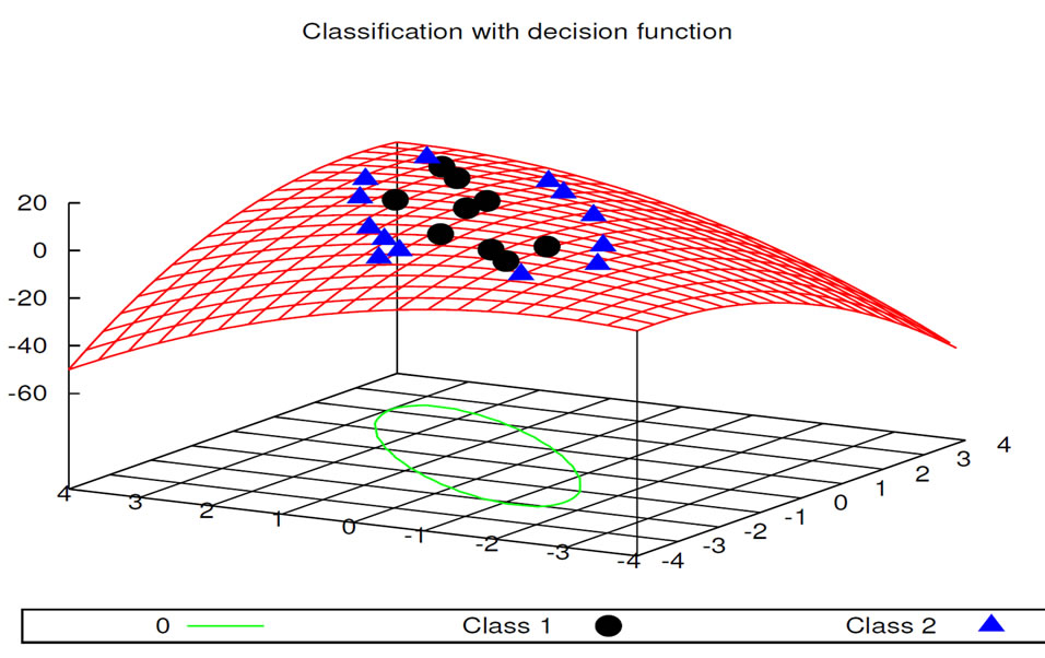
Figure 5. The transformation of the feature space.
known datasets which so far include uncovered areas of the feature space.
4.2. Second Experiment
! The second experiment is based on the well-known spiral dataset [11,17]. The problem in distinguishing two intertwined spirals is a non-trivial one. Figure 6 depicts the 970 patterns that form the two intertwined spirals. These patterns were provided in [17].
This experiment is an example of the way in which additional human expert knowledge can improve the quality of the found solutions (Section 3). For a human expert it is obvious that the problem is periodic. Therefore, to find good and short models it is essential to add periodic and trigonometric base functions. Without the trigonometric base functions learning algorithms have enormous problems in modeling the dataset [18]. Therefore, we allowed the algorithm to use addition (add), subtraction (sub), division (div), multiplication (mul, sin, cos) and all real numbers. Several correct problem solving solutions had been found by our system for this classification problem. One of them is Formula (3) (the numbers in the formula are rounded using 3 fractional digits) which is able to classify the spiral dataset without an error and Figure 7 shows the three-dimensional plot of the function. To the best of our knowledge it is one of the shortest known solutions that solve this classification task.
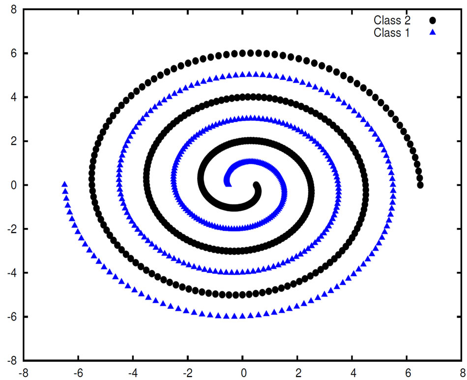
Figure 6. The spiral dataset.

Figure 7. The three-dimensional plot of function 3.
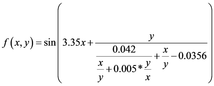 (3)
(3)
4.3. Real Life Dataset—Haberman’s Survival Dataset
The Habermans’s Survival dataset contains cases from a medical study that was conducted between 1958 and 1970 at the University of Chicago’s Billings Hospital on the survival of patients who had undergone breast cancer surgery [19-22].
It consists of 4 attributes:
1. Age of patient at time of operation (age)
2. Patient’s year of operation (the year of the operation)
3. Number of positive axillary nodes detected (nodes)
4. The survival status (class attribute)
Table 1 summarizes the rules of the pareto front of
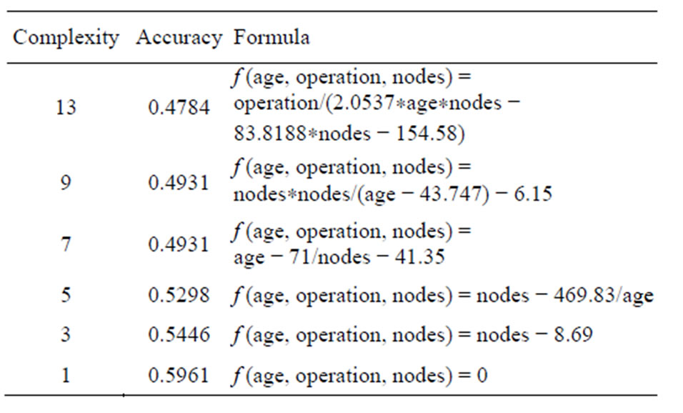
Table 1. Rules.
one run found by our Symbolic Regression system [11]. The formulas are ordered by complexity. It should be mentioned that repeating this procedure can result in different solutions (Section 3).
As a simple showcase to point out how additional insights into a domain can be gained we consider the formula f (age, operation, nodes) = age − 71/nodes − 41.35 which has a complexity of 7 in Table 1. It can be reformulated by age = 71/nodes + 41.35. A human user knows that the number of axillary nodes cannot have negative values. This implies that if the age of the patient is less than 41.35 the survival status is greater than 50 percent. This simple example shows, that reformulating and adding additional domain knwoledge adds further insight. New knowledge is derived and it can be used in another context. This procedure is, however, only possible on the basis of the symbolic and interpretable representation of the formulas (Section 2).
REFERENCES
- R. O. Duda, P. E. Hart and D. G. Stork, “Pattern Classification,” 2nd ed., Wiley Interscience, Hoboken, 2000.
- R. E. Steuer, “Multiple Criteria Optimization: Theory, Computations, and Application,” John Wiley & Sons, New York, 1986.
- J. K. Kishore, L. M. Patnaik, V. Mani and V. K. Agrawal, “Application of Genetic Programming for Multicategory Pattern Classification,” IEEE Transactions on Evolutionary Computation, Vol. 4, No. 3, 2000, pp. 242-258. doi:10.1109/4235.873235
- D. Robinson, “Implications of Neural Networks for How We Think about Brain Function,” Behavioral and Brain Science, Vol. 15, 1992, pp. 644-655.
- J. H. Holland, K. J. Holyoak, R. E. Nisbett and P. R. Thagard, “Induction: Processes of Inference, Learning, and Discovery,” Cambridge, 1989.
- P. Smolensky, “On the Proper Treatment of Connectionism,” Behavioral and Brain Sciences, Vol. 11, No. 1, 1988, pp. 1-74. doi:10.1017/S0140525X00052432
- T. S. Erfani and S. V. Utyuzhnikov, “Directed Search Domain: A Method for Even Generation of Pareto Frontier in Multiobjective Optimization,” Journal of Engineering Optimization, Vol. 43, No. 5, 2011, pp. 1-18. doi:10.1080/0305215X.2010.497185
- D. A. Freedman, “Statistical Models: Theory and Practice,” Cambridge University Press, Cambridge, 2005. doi:10.1017/CBO9781139165495
- M. O’Neill and C. Ryan, “Grammatical Evolution: Evolutionary Automatic Programming in an Arbitrary Language,” Kluwer Academic Publishers, Dordrecht, 2003.
- J. R. Koza, “Genetic Programming: On the Programming of Computers by Means of Natural Selection,” MIT Press, Cambridge, 1992.
- I. Schwab and N. Link, “Reusable Knowledge from Symbolic Regression Classification,” Genetic and Evolutionary Computing (ICGEC 2011), 2011.
- W. McCulloch and W. Pitts, “A Logical Calculus of the Ideas Immanent in Nervous Activity,” Bulletin of Mathematical Biophysics, Vol. 5, No. 4, 1943, pp. 115-133. doi:10.1007/BF02478259
- M. Kotanchek, G. Smits and A. Kordon, “Industrial Strength Genetic Programming,” In: R. Riolo and B. W. Kluwer, Eds., GP Theory and Practice, 2003.
- G. Smits and M. Kotanchek, “Pareto-Front Exploitation in Symbolic Regression,” In: R. Riolo and B. W. Kluwer, Eds., GP Theory and Practice, 2004.
- M. Schmidt and H. Lipson, “Discovering a Domain Alphabet,” Genetic and Evolutionary Computation Conference (GECCO’09), 2009, pp. 1083-1090. doi:10.1145/1569901.1570047
- T. Hastie, R. Tibshirani and J. Friedman, “The Elements of Statistical Learning: Data Mining, Inference, and Prediction,” Springer-Verlag, New York, 2001.
- K. Lang and M. Witbrock, “Learning to Tell Two Spirals Apart,” Proceedings of 1988 Connectionists Models Summer School, San Mateo, 1989, pp. 52-59.
- R. Setiono, “A Neural Network Construction Algorithm Which Maximizes the Likelihood Function,” Connection Science, Vol. 7, No. 2, 1995, pp. 147-166. doi:10.1080/09540099550039327
- S. J. Haberman, “Generalized Residuals for Log-Linear Models,” Proceedings of the 9th International Biometrics Conference, Boston, 1976, pp. 104-122.
- J. M. Landwehr, D. Pregibon and A. C. Shoemaker, “Graphical Models for Assessing Logistic Regression Models,” Journal of the American Statistical Association Vol. 79, No. 385, 1984, pp. 61-83. doi:10.1080/01621459.1984.10477062
- W. D. Lo, “Logistic Regression Trees,” Ph.D. Dissertation, Department of Statistics, University of Wisconsin, Madison, 1993.
- A. Frank and A. Asuncion, “UCI Machine Learning Repository,” 2010. http://archive.ics.uci.edu/ml