Open Journal of Acoustics
Vol.3 No.4(2013), Article ID:40574,10 pages DOI:10.4236/oja.2013.34017
Finite Element Analysis of Sound Transmission Loss in One-Dimensional Solids
Department of Mechanical and Industrial Engineering, Ryerson University, Toronto, Canada
Email: *syu@ryerson.ca
Copyright © 2013 S. D. Yu, J. G. Kawall. This is an open access article distributed under the Creative Commons Attribution License, which permits unrestricted use, distribution, and reproduction in any medium, provided the original work is properly cited.
Received October 4, 2013; revised November 4, 2013; accepted November 11, 2013
Keywords: finite element method; sound transmission loss
ABSTRACT
A higher-order acoustic-displacement based finite element procedure is presented in this paper to investigate one-dimensional sound propagation through a solid and the associated transmission loss. The acoustic system consists of columns of standard air and a solid, with the upstream column of air subjected to a sinusoidal sound source. The longitudinal wave propagation in each medium is modeled using three-node finite elements. At the interfaces between the air and the solid medium, the continuity in acoustic displacements and the force equilibrium conditions are enforced. The Lagrange multipliers method is utilized to assemble the global equations of motion for the acoustic system. Numerical results obtained for various test cases using the procedure described in the paper are in excellent agreement with the analytical solutions and other independent solutions available in the literature.
1. Introduction
In general, a noise control problem deals with three elements—source, path, and receiver. The most effective means of controlling noise is to reduce the noise generated at the source. However, it is not always possible to attain an acceptable level of noise by this means alone. It is often necessary to attenuate as much sound energy as possible along its path from the source to the receiver. When efforts to reduce noise at its source or along the path of transmission are insufficient, measures such as using ear plugs and limiting exposure time can be used to protect the receiver.
This paper is concerned with a displacement-based finite element method (FEM) formulation of one-dimensional sound propagation through solids and the application of the methodology to determine the sound transmission loss associated with these structures. The main advantages of using the displacement FEM formulation, compared to the pressure-based variational approach by Gladwell [1] and Craggs [2], are: 1) the analysis can be easily formed for both transient and steady-state situations in the real domain, 2) Hamilton’s variational principle can be used to derive equations of motion and boundary conditions, and 3) interface conditions between two distinct media can be handled using Lagrange multipliers in a generic manner without identifying the direction of wave propagation, namely, forward and backward, or transmitted and reflected.
Isoparametric finite elements are generally used for sound propagation problems (Craggs [3], Kang and Bolton [4]). However, in the present work, to enhance the computational efficiency for dynamical problems and ease in handling interface conditions between two distinct media, three-node higher-order (non-isoparemetric) finite elements are used to examine wave propagation in one-dimensional acoustic systems consisting of various distinct media. Six nodal quantities—the variable and its derivative (i.e., gradient) at all three nodes—are introduced for the element acoustic displacement vector. Thus, each three-node, higher-order, finite element has 6 nodal acoustic displacements. Moreover, quintic polynomials are used as the interpolation function for the acoustic displacement within an element. This feature is especially important when dealing with large wave numbers, e.g., in the case of high frequency sound propagating in an extended medium. Since formulation of interface conditions generally requires both the field variable and its gradient, it is natural to introduce gradients into the analysis.
When sound propagation in different media is studied by means of finite element analysis, it is often necessary to formulate and implement interface conditions. According to Craggs [3], when two systems are linked together, it may be assumed that there exists an incompressible fluid boundary layer, i.e., a small volume of incompressible fluid adjacent to the interfacial node. The dimensions of this volume are small compared with the acoustic wavelength. This may be interpreted as the two media having continuous acoustic displacements and balanced acoustic pressures across the boundary layer. With acoustic displacement as the field variable, these two conditions can be easily implemented. In a one-dimensional situation, the pressure on either side of the boundary layer can be related to the displacement gradient (or acoustic strain) through compressibility, for fluids, and modulus of elasticity, for solids. When writing the two interface conditions in terms of nodal variables on the two sides of the boundary layer, the Lagrange multipliers method (Tabarrok and Rimrott [5]) may be used for assembly of the global equations of motion for an acoustic system having multiple media.
The conceptual model proposed by Morse and Ingard [6] has been modified by Craggs [7] through introduction of the structure factor, porosity, and resistivity, for application of the generalized Rayleigh model to a sound absorbing material. The properties of sound absorption and reaction of materials can be modeled by using equivalent density, equivalent compressibility, and resistivity in the wave equation.
The objective of this paper is to present a finite element procedure for computing the sound transmission loss in solids using acoustic displacement as the field variable. Although the wave equation considered herein is one-dimensional, the procedure can be extended to twoand three-dimensional problems.
2. Mathematical Procedure
In this section, the equations of motion of the one-dimensional acoustic system depicted in Figure 1 are presented using an inertial coordinate system. The origin of the coordinate system is located at the inner surface of the rigid vibrating piston when the axial displacement of the piston is zero. For the purpose of studying the sound absorption and the sound transmission loss through a solid or porous medium, it is assumed that sound waves either terminate at the right end of the tube or are transmitted to the ambient air, although different boundary conditions may be imposed.
2.1. Variational Principle
In modeling the one-dimensional acoustic system shown
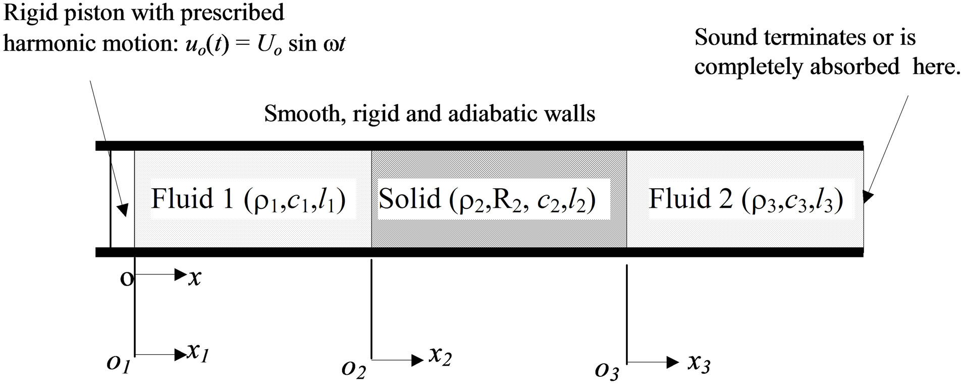
Figure 1. A one-dimensional system having three media for studying sound transmission loss.
in Figure 1, the following assumptions are made: 1) there is no ambient fluid flow; 2) heat transfer associated with acoustic waves is negligible everywhere; 3) the fluids are inviscid; 4) the tube walls surrounding the three media are smooth, rigid, and adiabatic; 5) the cross section of each medium is much smaller in size than its length. With the help of these assumptions, the wave propagation in each medium is linear.
For a column of solid or porous material, the longitudinal displacement or acoustic displacement is used as the field variable for consistency. And once the displacement field is obtained, the velocity and stress inside the material may be obtained. For a column of fluid (air) without flow, the plane acoustic wave equation may be formulated using one of the three field variables—acoustic displacement, acoustic velocity, and acoustic pressure. In this paper, the acoustic displacement is chosen as the field variable. And once the acoustic displacement is determined, the acoustic velocity and pressure everywhere in the fluid may be determined.
To derive the wave equations for a system of multiple media, we first study a single, unconstrained (one-dimensional) medium. The relevant acoustic material and geometric properties are density , speed of wave propagation
  or modulus of elasticity for solids or compressibility for fluids, damping coefficient per unit of crosssectional area
  for solids or resistivity for porous materials, length
 , and cross-sectional area
 . According to Hamilton’s principle, the equations of motion for the single medium may be obtained from
 (1)
(1)
In Equation (1),  is the Lagrangian, defined as
 , where
  is the kinetic energy and
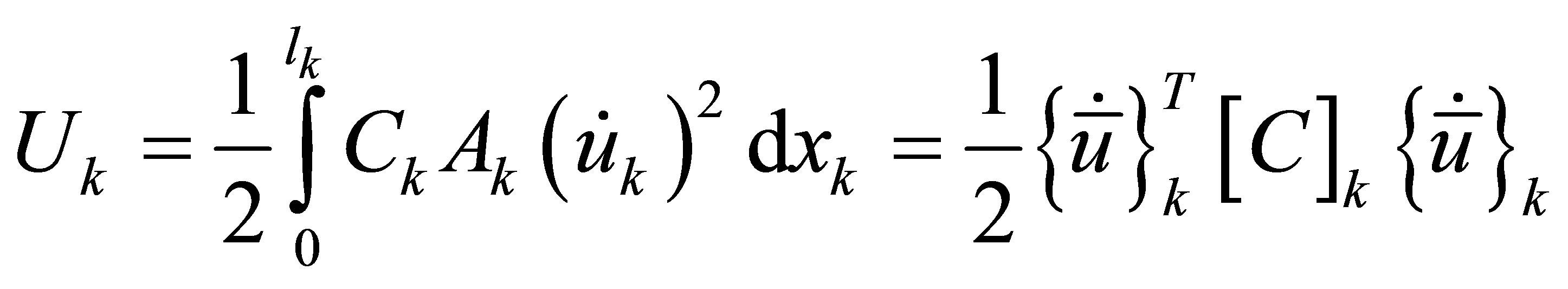
  is the potential energy;
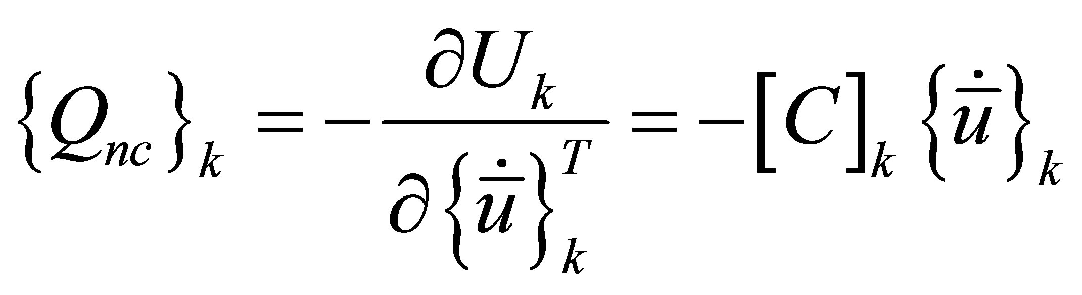
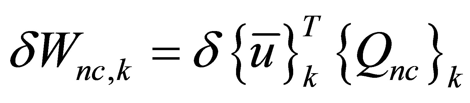
  is the virtual work done by distributed non-conservative forces and the distributed damping force;
  is the longitudinal acoustic displacement; subscript k refers to the k-th medium or system component; t is time.
In acoustics, the wave equations are often written in a different form (Crocker [8]). However, in a finite element analysis, it is preferable to use the acoustic displacement as the field variable because Hamilton’s variational principles can be used to derive the ordinary differential equations for transient and steady state responses of an acoustic system to excitations.
2.2. Finite Element Formulations for a System Component
Suppose that a system component (a fluid, solid or porous medium) is modeled using  three-node one-dimensional finite elements, as depicted in Figure 2. Within each finite element, the acoustic displacement,
  , varies with the local axial coordinate,
  , as
, as
 (2)
(2)
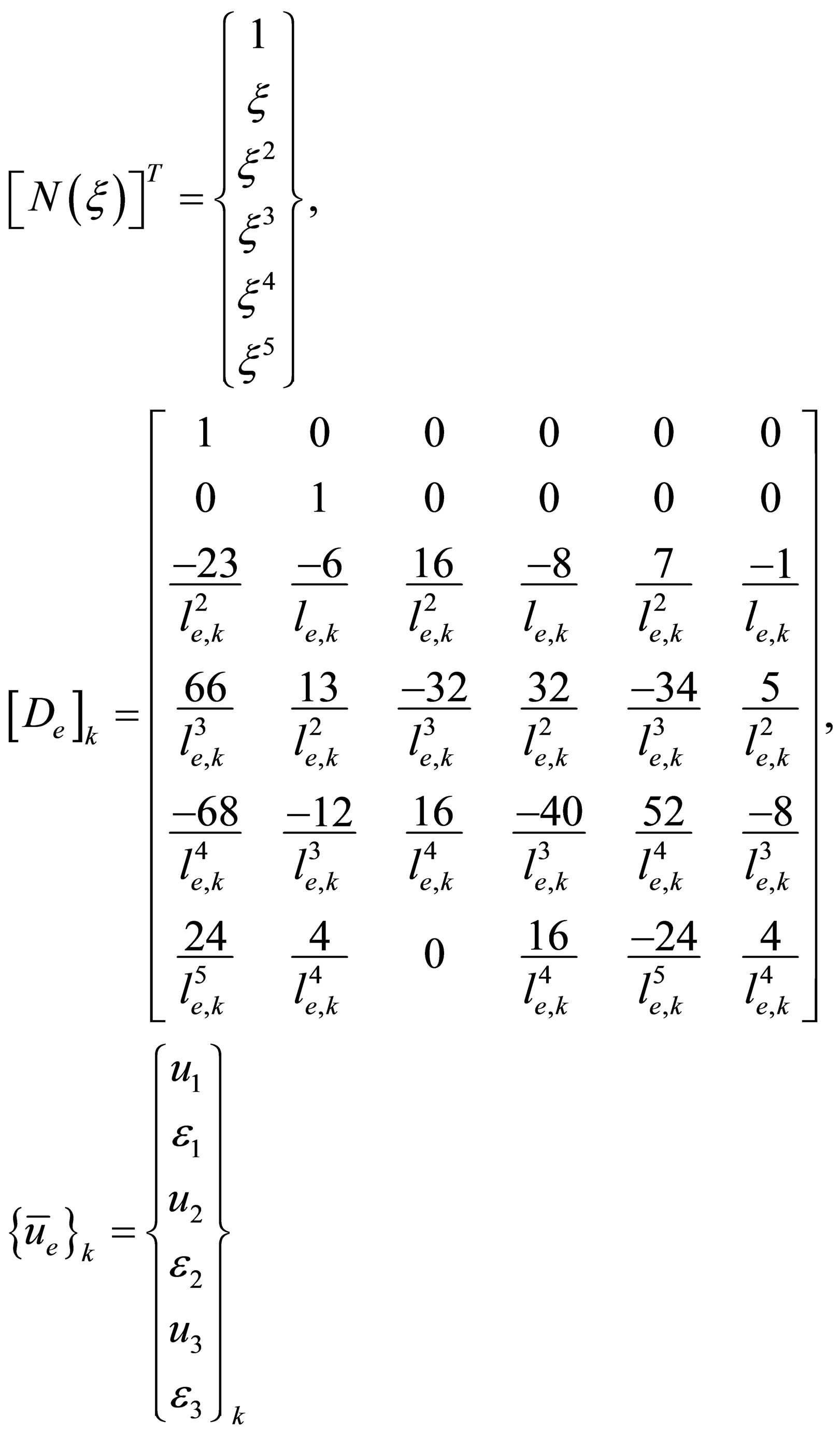
where 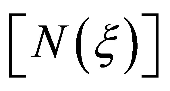 is the shape function matrix;
 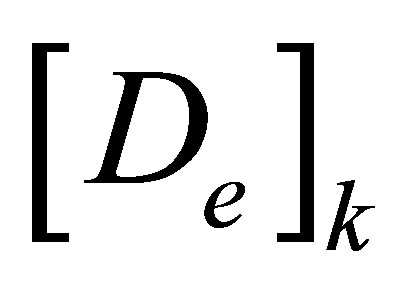 is the element geometric matrix, and
 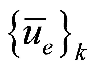 is the element nodal displacement vector. These quantities are defined as follows
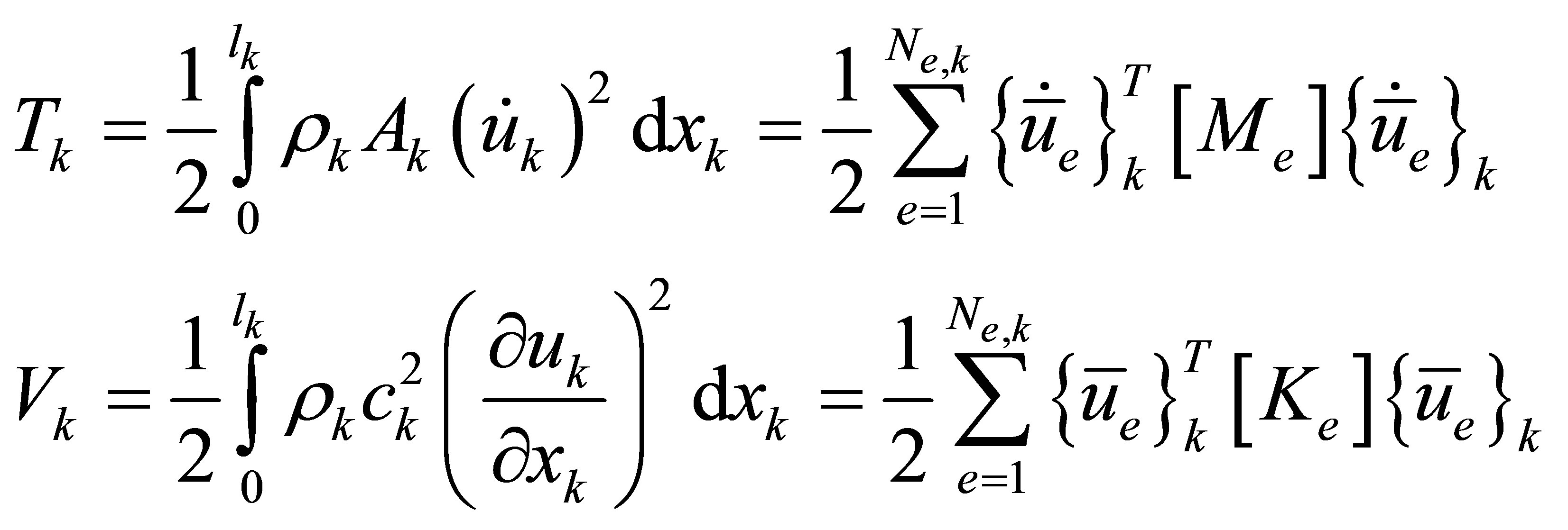 (3)
(3)
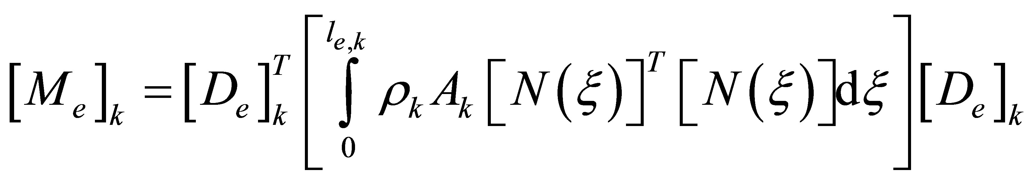
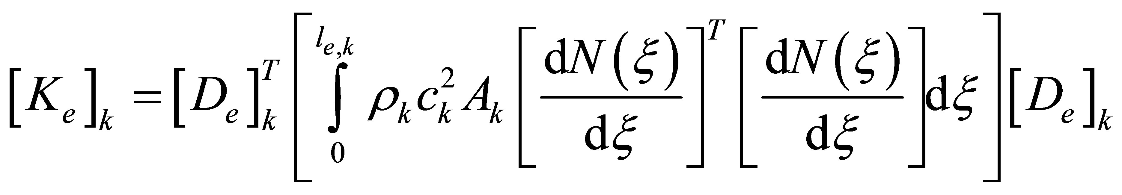
where the element mass and element stiffness matrices,
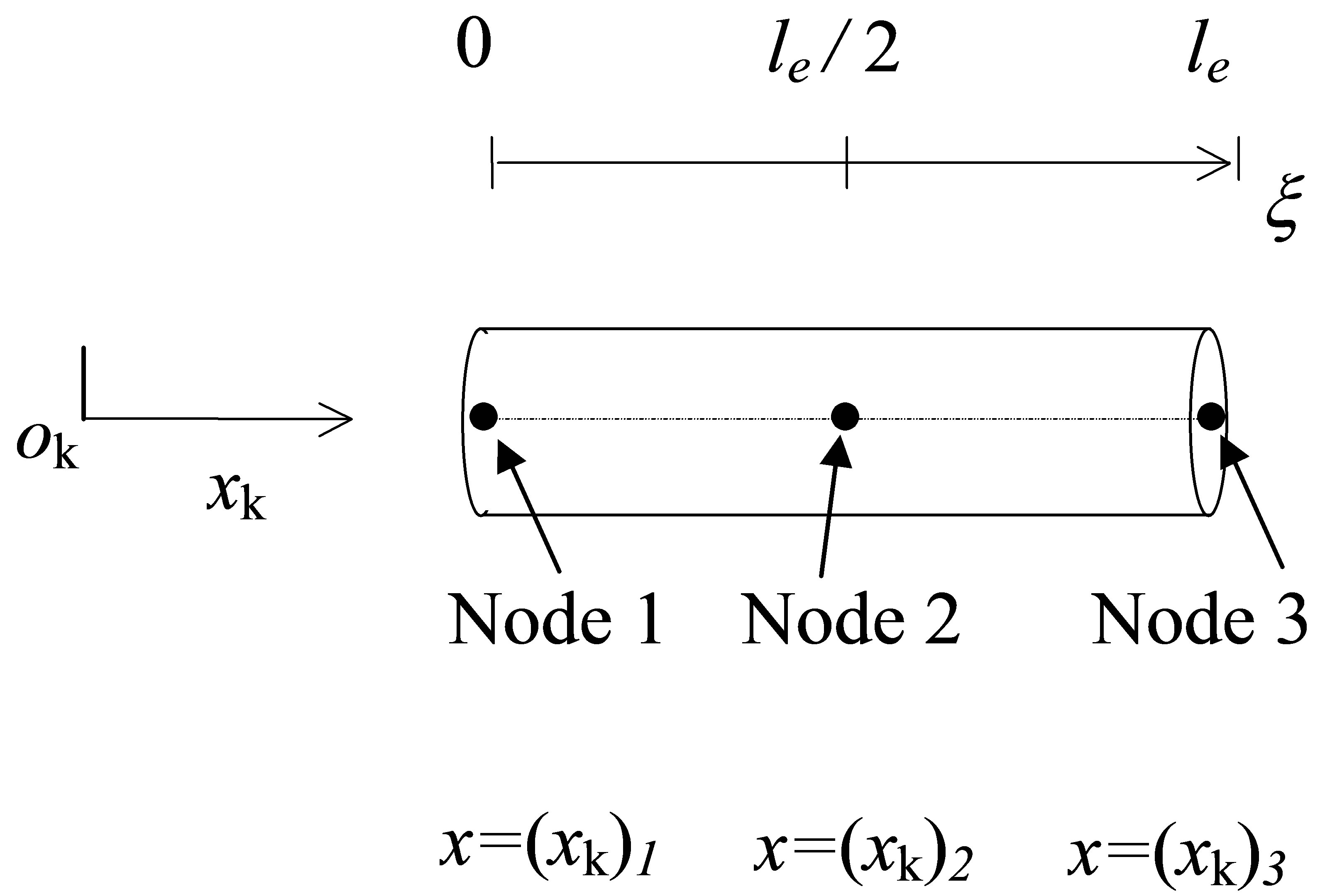
Figure 2. A three-node finite element for component k and its coordinates.
 and
and , are given by
To complete the kinetic and potential energies, the following component nodal displacement vector is introduced
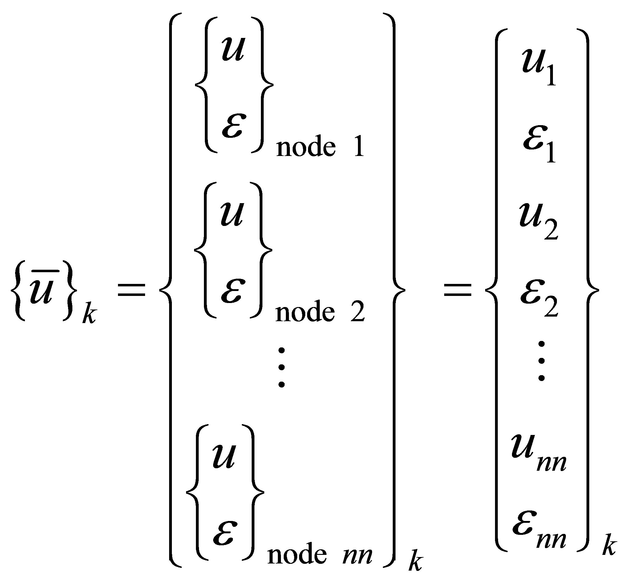 (4)
(4)
where nn appearing in the above equation as subscripts represents the number of nodes in a finite element mesh for component k.
Once the strategy for formulating the component nodal vector is determined, the element displacement vector may be related to the component displacement vector by a transformation matrix,  , as follows
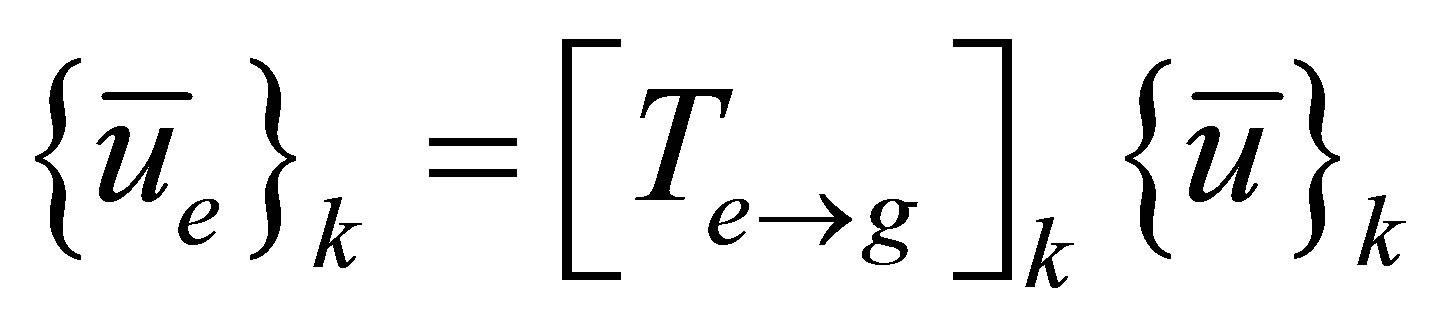 (5)
(5)
Utilizing the transformation in Equation (5), the component kinetic and potential energies may be written as
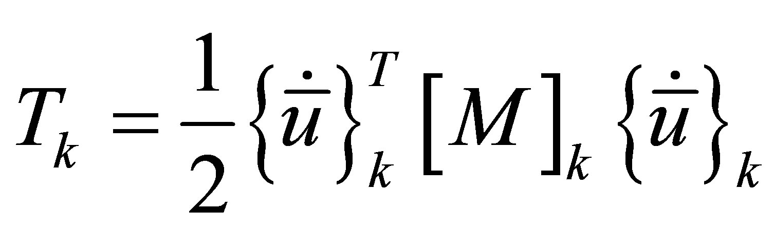 (6)
(6)
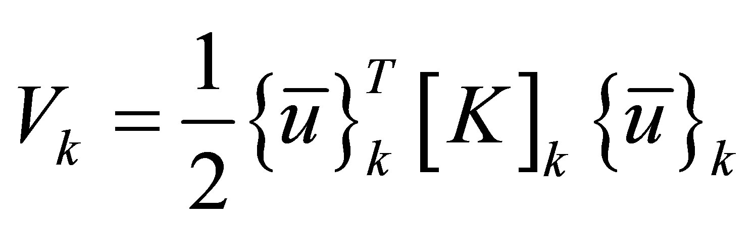
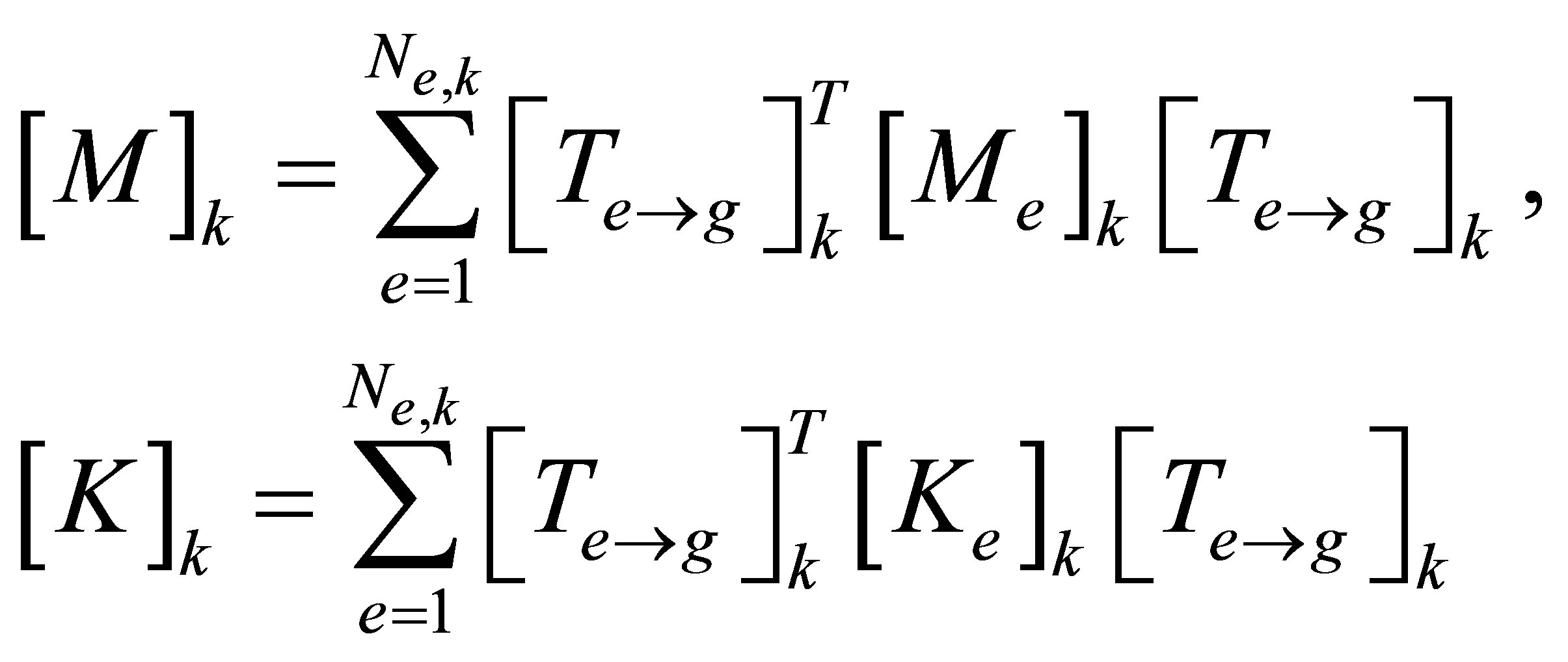
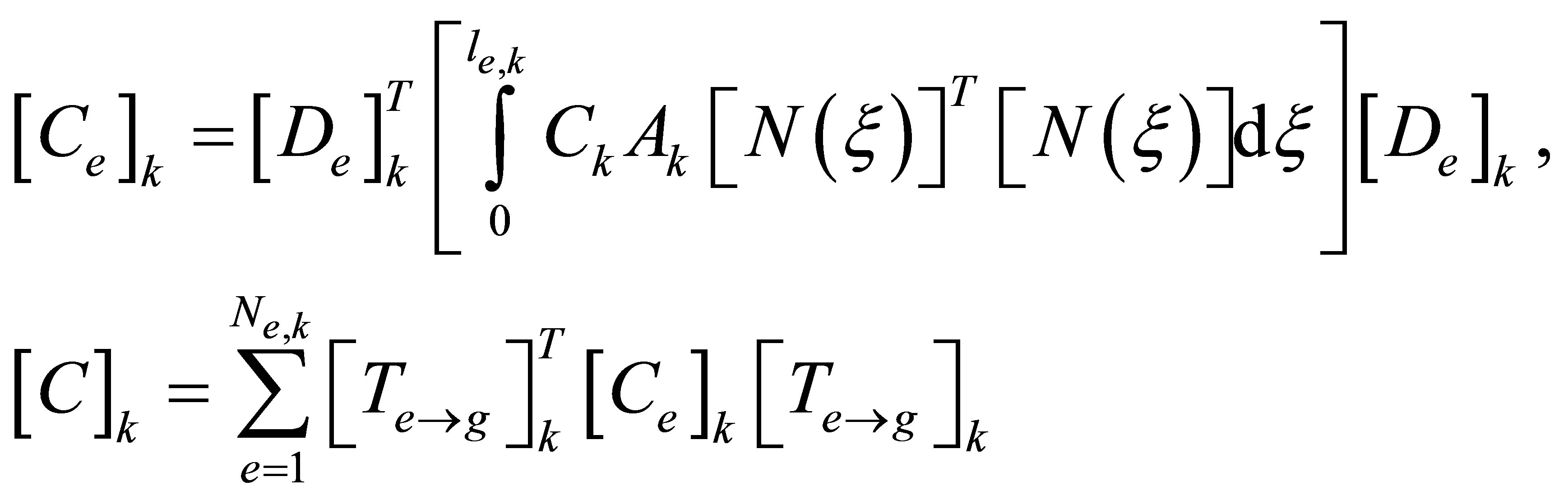
where the component mass and stiffness matrices are defined by
When damping is present in the component, the distributed damping (non-conservative) force will do work. For Rayleigh damping, the effect can be considered through a Rayleigh damping function,  , defined as
 (7)
(7)
where  is the damping coefficient;
  is the damping matrix, which can be obtained from the following equations
For a Rayleigh material, the generalized damping force vector may be derived from the following relations
 (8)
(8)
The work done by the generalized force vector for a virtual displacement  is
is
 (9)
(9)
When the component nodal displacement vector is chosen as a set of generalized coordinates, it can be shown that satisfaction of Hamilton’s principle in Equation (1) yields the following Lagrange equations
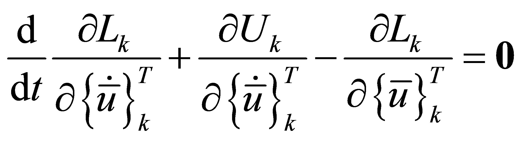 (10)
(10)
Substituting Equations (6) and (7) into Equation (10), one obtains the following equations of motion for an unconstrained component in terms of the component nodal displacement vector
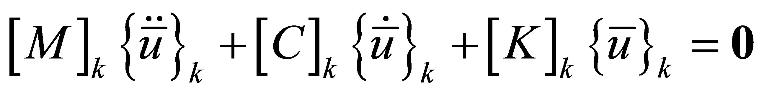 (11)
(11)
Since a component in a system interacts with its neighboring components, the above equations of motion are coupled through displacements at the interfacial nodes with other component equations and cannot be solved independently.
It is noted that the component equations of motion in Equation (11) may be obtained from the wave equation and Galerkin’s weak form of the variational principle when time t is held fixed or t is considered a parameter.
In this paper, we decided to treat the interface conditions between components using the Lagrange multipliers method, which is consistent with Hamilton’s principle and the Lagrange equations method.
2.3. Boundary Conditions
The natural boundary condition at either end of a component, according to Hamilton’s principle, is either 1) the acoustic displacement is prescribed or 2) the acoustic pressure is zero. The prescribed displacement includes the situations where the boundary moves with a rigid piston (the source of sound) and where sound propagation terminates. The zero acoustic pressure is rarely encountered for a component of finite size. Besides the two natural boundary conditions, non-natural boundary conditions may also be imposed. For example, a sound absorption material or structure may be modeled as boundary conditions when only the reflection or transmission at the sound-structure interface is of interest. These boundary conditions may include inertial, stiffness and damping elements.
When one end of a column of fluid, say, the left end of fluid 1, as shown in Figure 1, adheres to a rigid and vibrating piston with a prescribed acoustic velocity, the acoustic velocity at the first node must be specified and equal to that of the piston. For harmonic acoustic excitation of a single frequency, the prescribed acoustic velocity may be written as
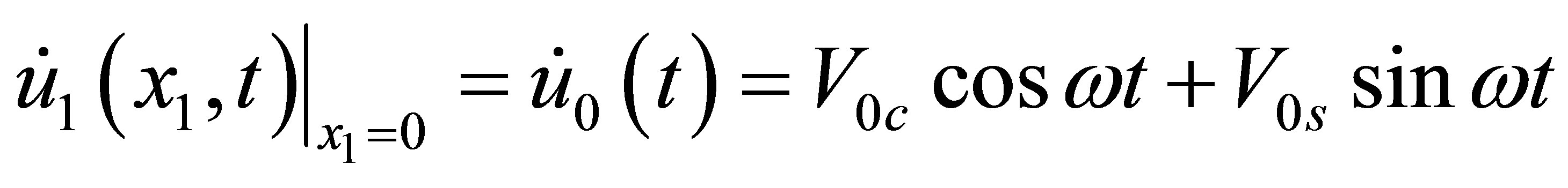 (12)
(12)
where  and
and  are the cosine and sine components of the harmonically varying velocity;
  is the excitation frequency. In this paper, as the acoustic displacement is adopted as the field variable, the equivalent sound source may be written in terms of the acoustic displacement as follows
 (13)
(13)
where  and
and .
.
2.4. Interface Conditions
At the interface between the components, it is assumed that 1) the acoustic displacements or velocities of the components at the two sides of a thin and incompressible boundary layer are identical in the direction normal to the interface, and 2) the acoustic pressures at the two sides of the boundary layer are also identical. These two conditions ensure the continuity and force balance across a thin boundary layer. For the acoustic system with three components, there exist two interfaces and four interface conditions. Using local coordinates, these conditions may be written as
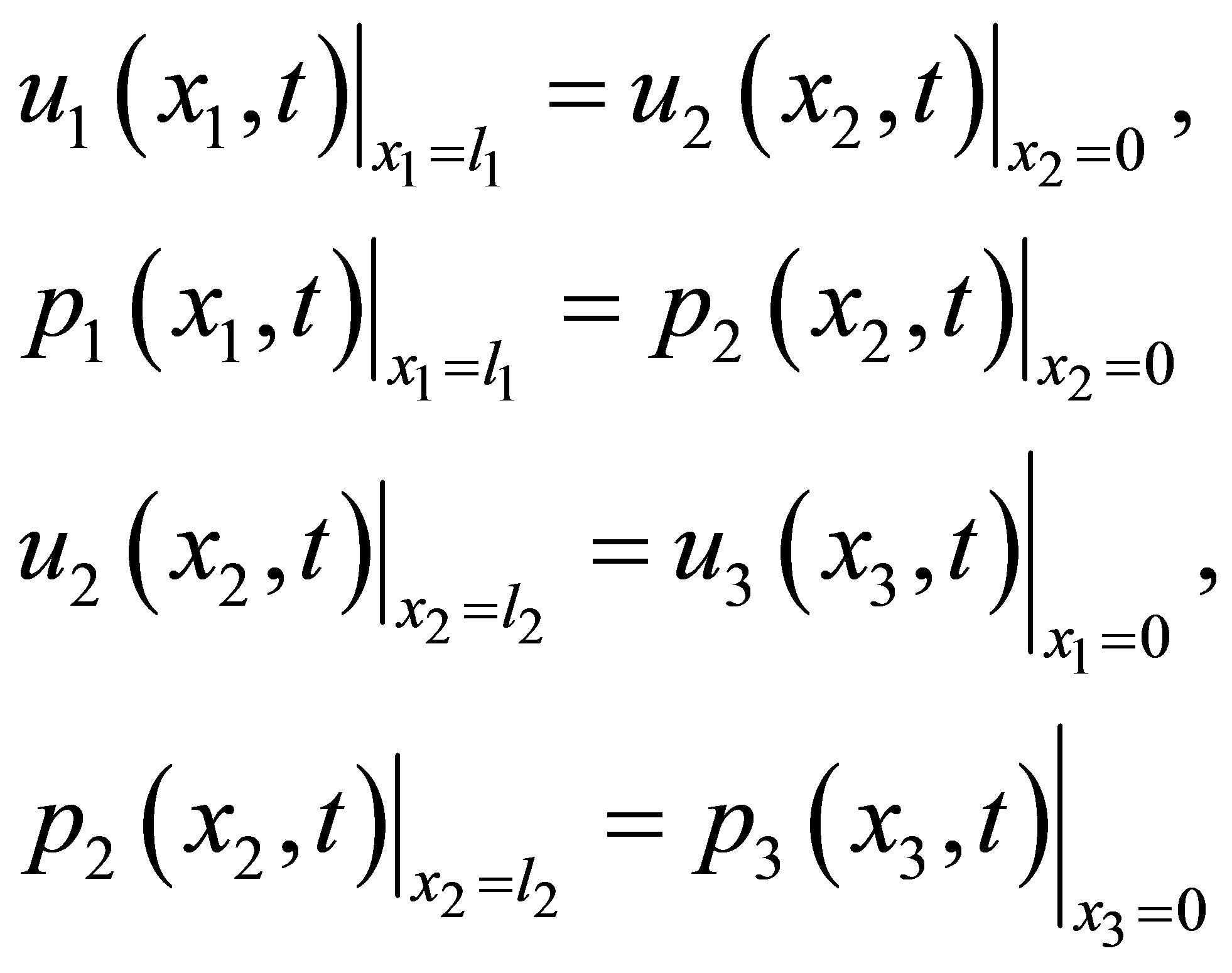 (14)
(14)
For a fluid or solid, the acoustic pressure and displacement are related by
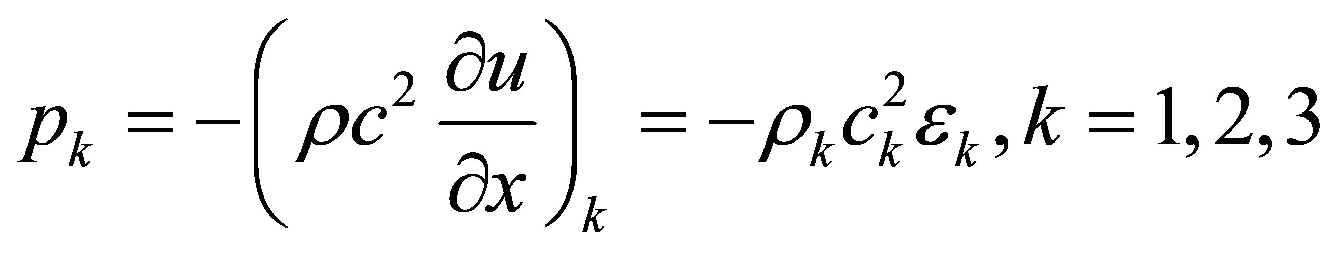 (15)
(15)
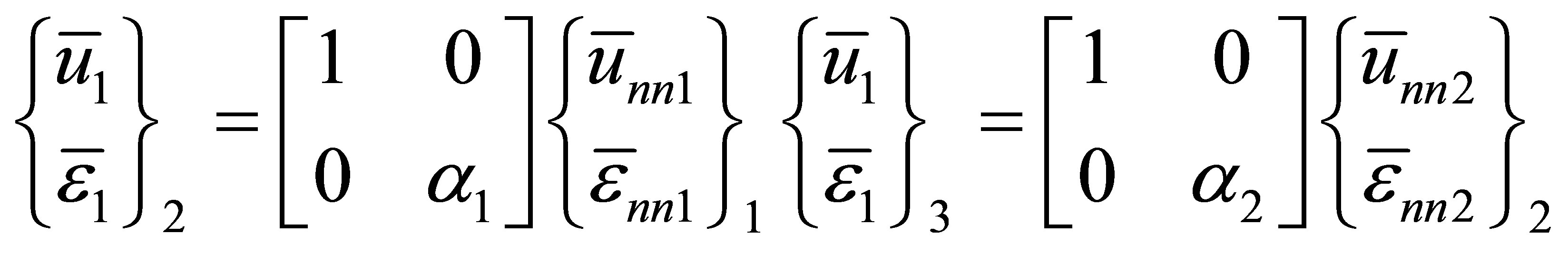
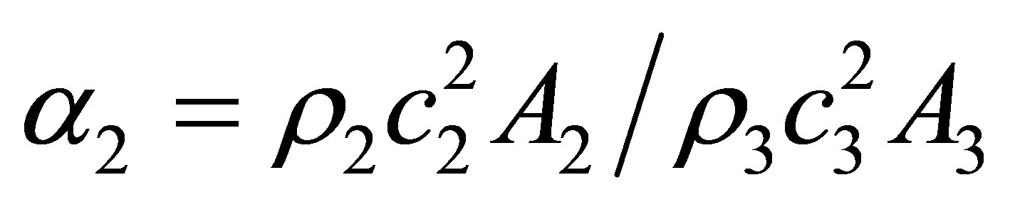
Substituting Equation (15) into Equation (14), the four interface conditions may be rewritten in terms of acoustic displacements and strains as
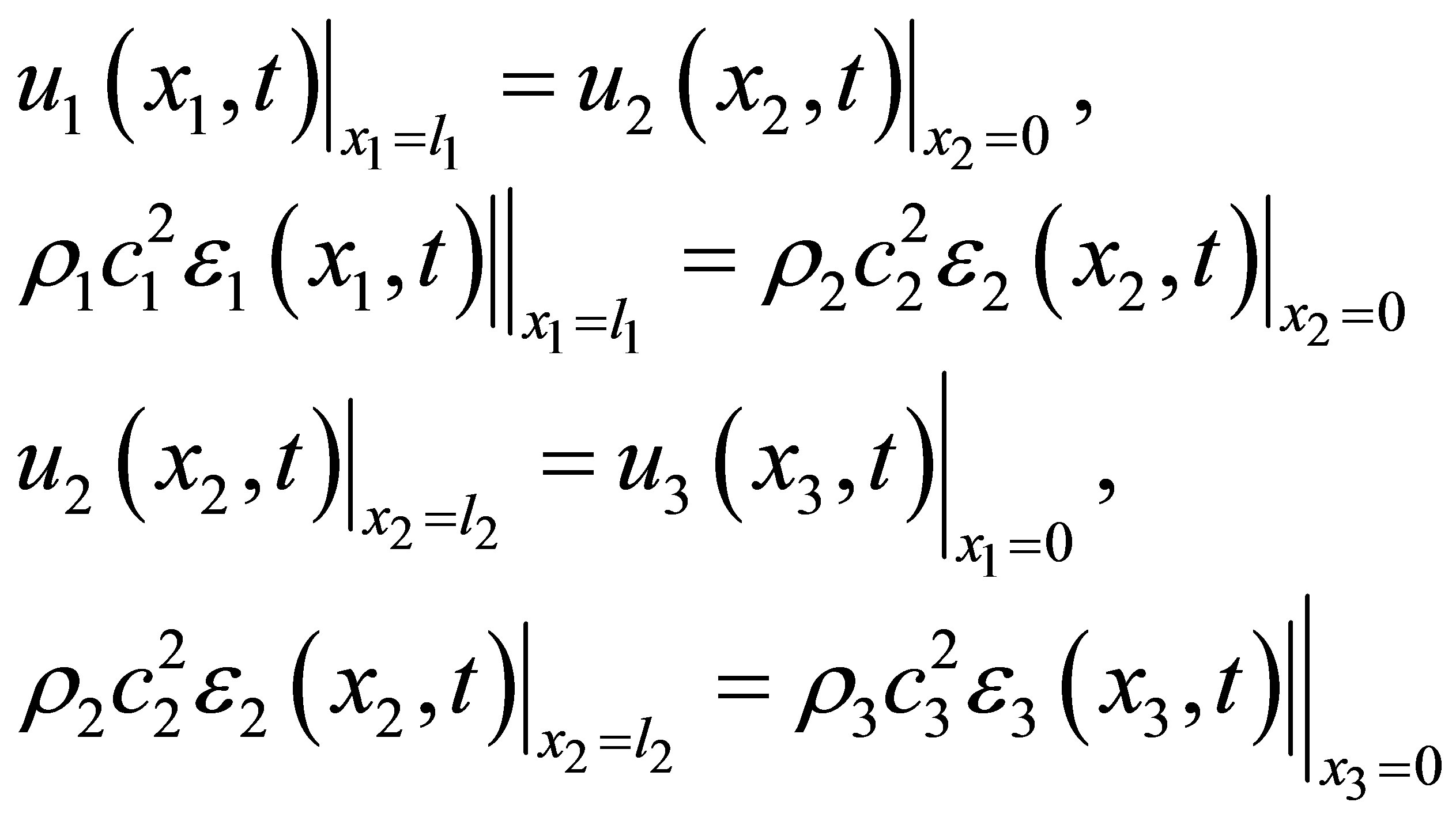 (16)
(16)
It must be pointed out that the interface conditions between two different media described in Equation (16) are valid for waves propagating in either direction (forward or backward; transmitted or reflected). The reason is that the sign of the acoustic pressure is also opposite to that of the acoustic strain. In other words, compression of a medium (negative strain) corresponds to a positive acoustic pressure; rarefaction of a medium (positive strain) corresponds to a negative acoustic pressure. However, when using acoustic velocity or pressure as the field variable, separate expressions are required for a wave propagating in different directions.
2.5. Assembly of Equations of Motion for the Acoustic System
With the neglect of the viscosity of the air on either side of the solid, the three sets of equations may be written as
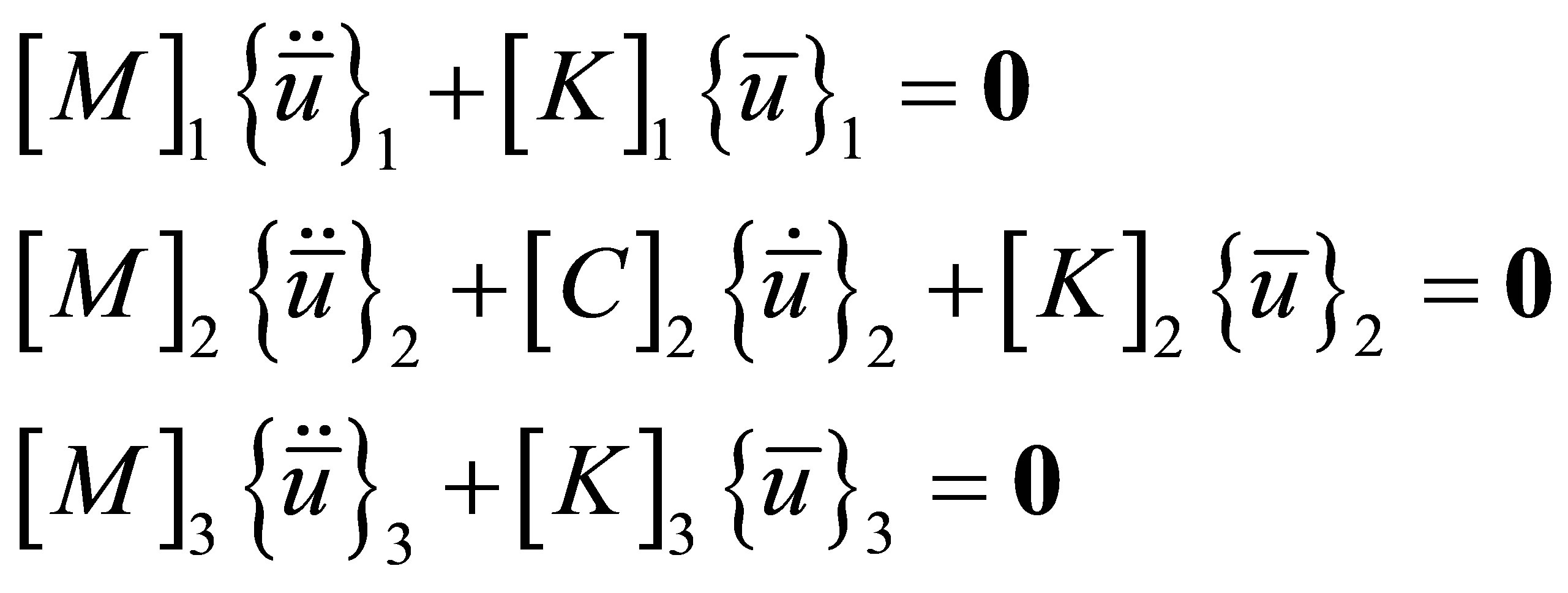 (17)
(17)
Based on the model for a porous material developed by Morse and Ingard [6] and Craggs [7], the following material properties of the solid can be calculated using the density of air , speed of sound in air
 , the structure factor
 , porosity
 , and resistivity
 (18)
(18)
To finalize the equations of motion for the acoustic system consisting of several components, each set of component equations in Equation (17) must be modified to satisfy the boundary and interface conditions. The first column of fluid is placed directly adjacent to the sound source; consequently, from Equation (13), the acoustic displacement of the first node of the first column of air must be equal to the piston displacement, or  .
.
If the air on the right side of the solid terminates at the right-most end of the system, the last node must have zero acoustic displacement, or . However, if the right end is exposed to the open air, the acoustic pressure is zero. This indicates that the acoustic strain must be zero, or
 . The two types of homogeneous boundary conditions may be easily handled by modifying the stiffness matrix using the penalty method.
Since the acoustic displacement of the first node is specified and not subjected to variation, the first equation for the air on the left side of the solid may be deleted. After implementing the prescribed acoustic movement at the left-most node, the modified equations of motion may be written as
 (19)
(19)
where  is the resulting matrix of
  after deleting the first row and first column;
  and
and  are the acoustic force vectors, defined by
To implement the boundary condition at the right-most end, the second to last diagonal element or the last diagonal element associated with  in
in  must be changed to
 . The modified equations of motion for the air on the right side of the solid are then written as
 (20)
(20)
where  is identical to
  except for element element (2nn-1, 2nn-1), or (2nn, 2nn). Values of
  (the largest number permitted by a computing machine) should be taken to make
  the only dominant term in the first equation of Equation (19) without causing overflow problems.
To illustrate how global equations of motion of the acoustic system are obtained from the equations of motion of all components, let us examine the four interface conditions, which are now written in the following matrix form
 (21)
(21)
or
 (22)
(22)
where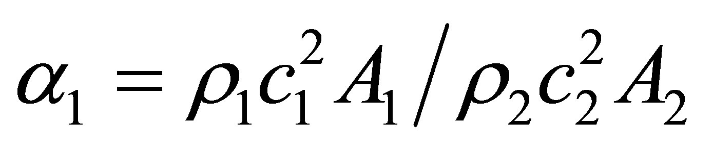 ;
; .
.
To implement the interface conditions in Equation (22) into the global equations of motion of the acoustic system, we introduce the following potential to the lagrangian
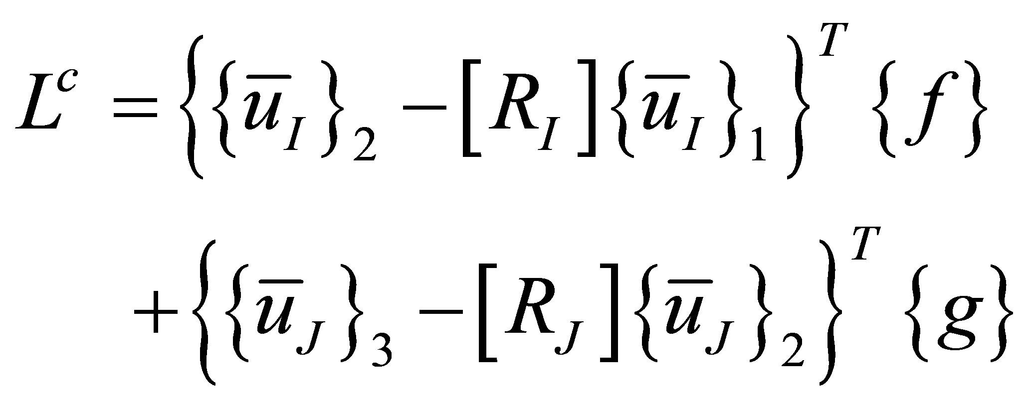 (23)
(23)
where {f} and {g} are constraint forces between two media at interfaces I and J, respectively.
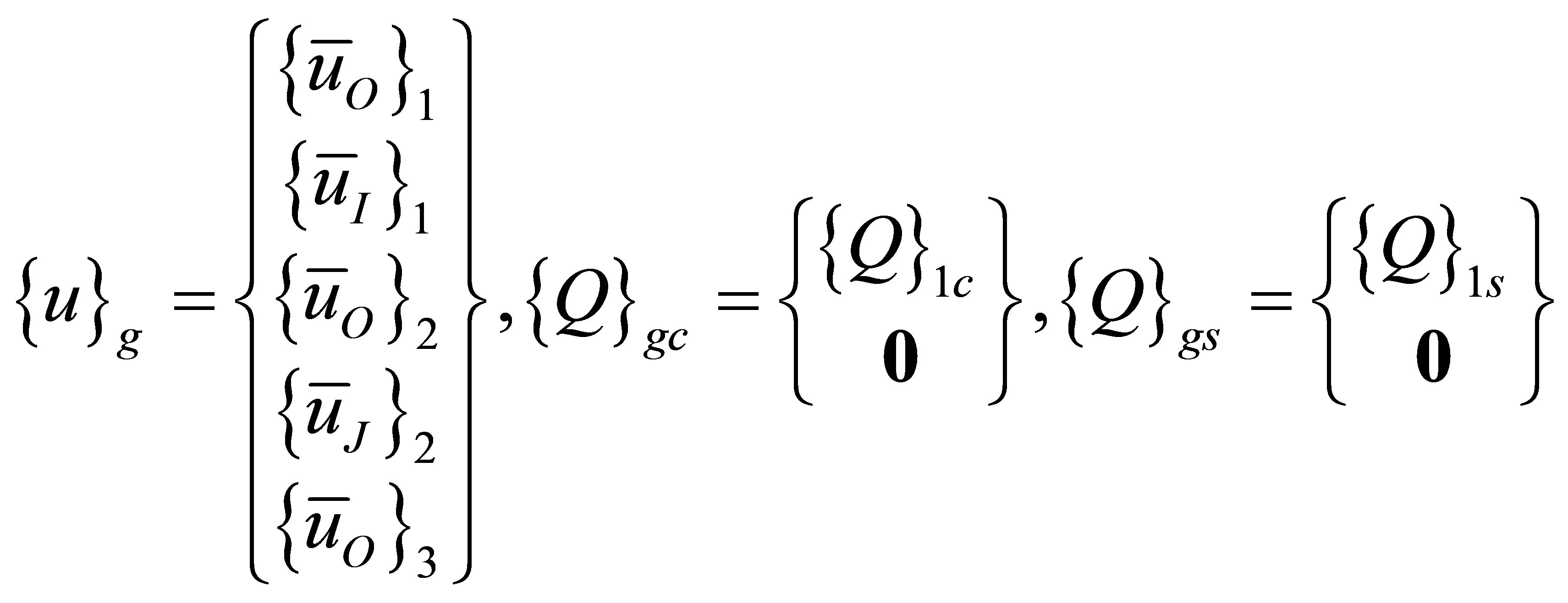
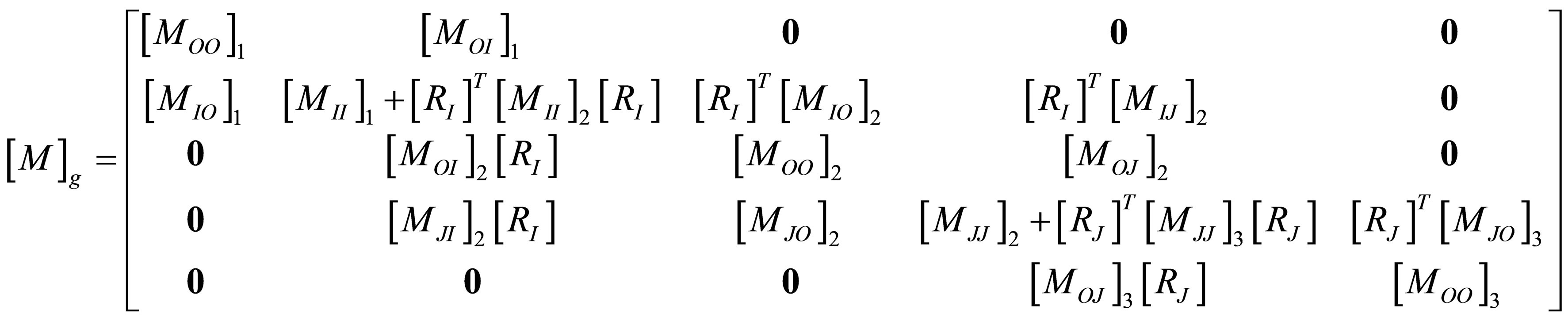
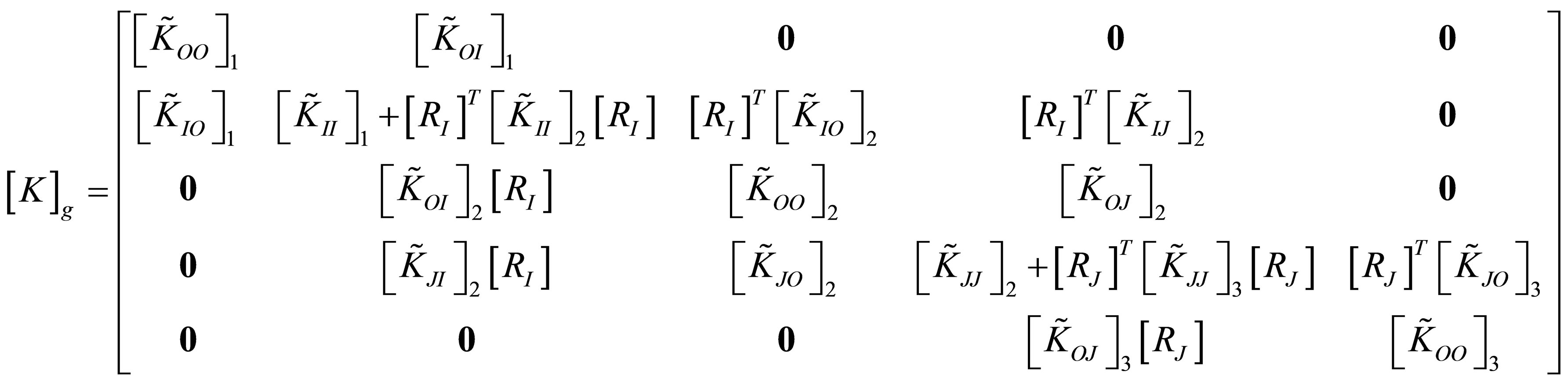
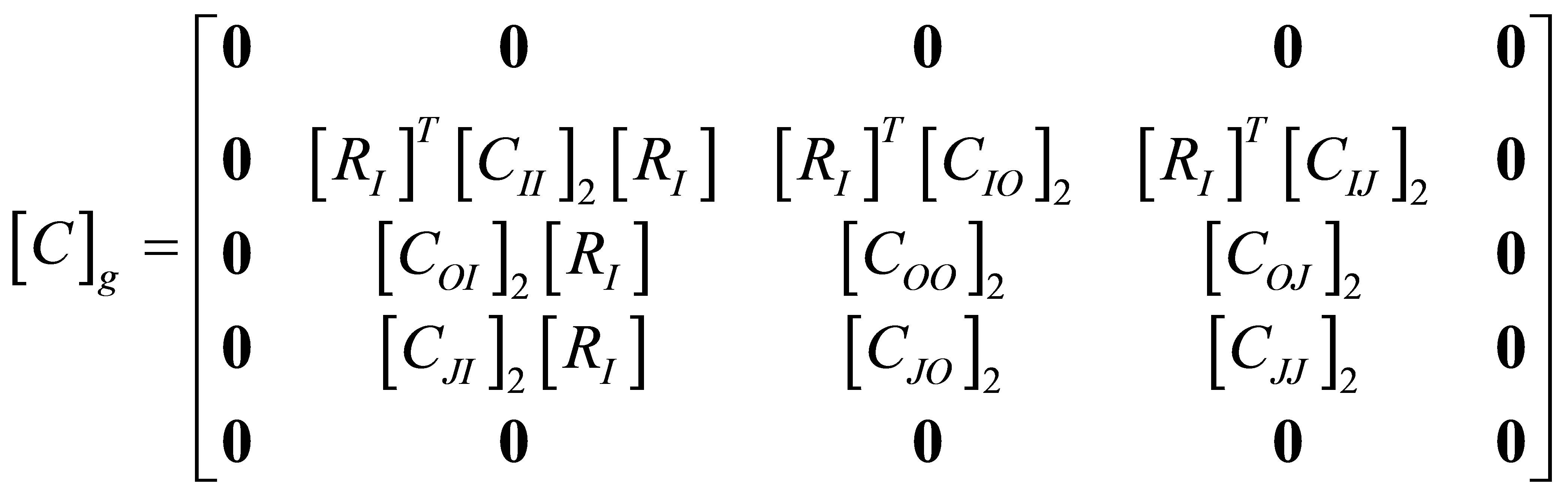
Incorporating the work done by constraint forces on arbitrary boundary displacements, the modified equations of motion in the desired partitioned form along with the constraint equations are written as
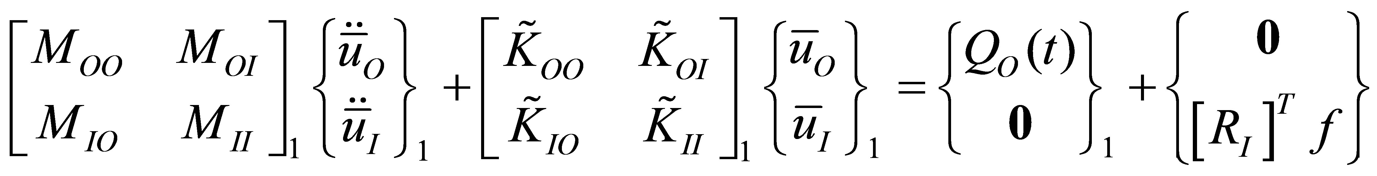 (24)
(24)
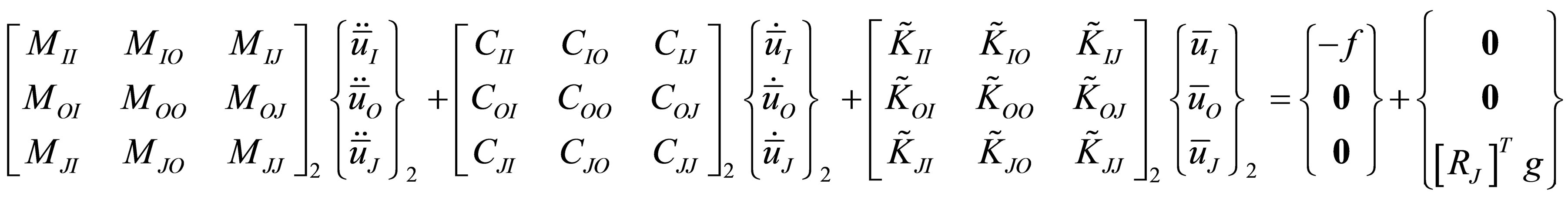 (25)
(25)
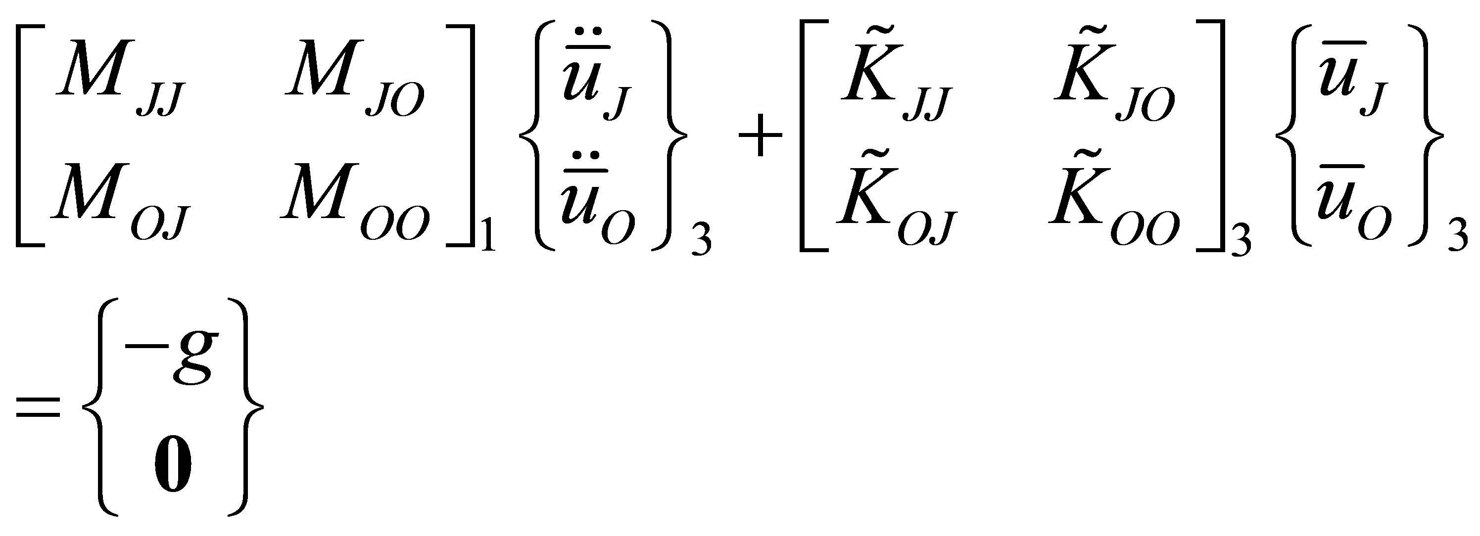 (26)
(26)
where subscripts O, I, J refer to interior, first interfacial and second interfacial degrees of freedom.
Equations (22), (24), (25) and (26) constitute a complete set of dynamical equations for acoustic displacements and constraining forces between two adjacent media. To obtain a system of second order ordinary differential equations, these equations are often revised by deleting the constraining force vectors. From Equation (22),  and
and  may be replaced with
  and
and , respectively, in Equations (24), (25) and (26). In addition, constraining force vectors {f} and {g} may also be deleted to form simple matrix operations. For example, vector {f} may be deleted by pre-multiplying the first set of equations in Equation (25) and then adding it to the second set of equations in Equation (24).
A set of inhomogeneous governing differential equations written in terms of the modified displacement vector as
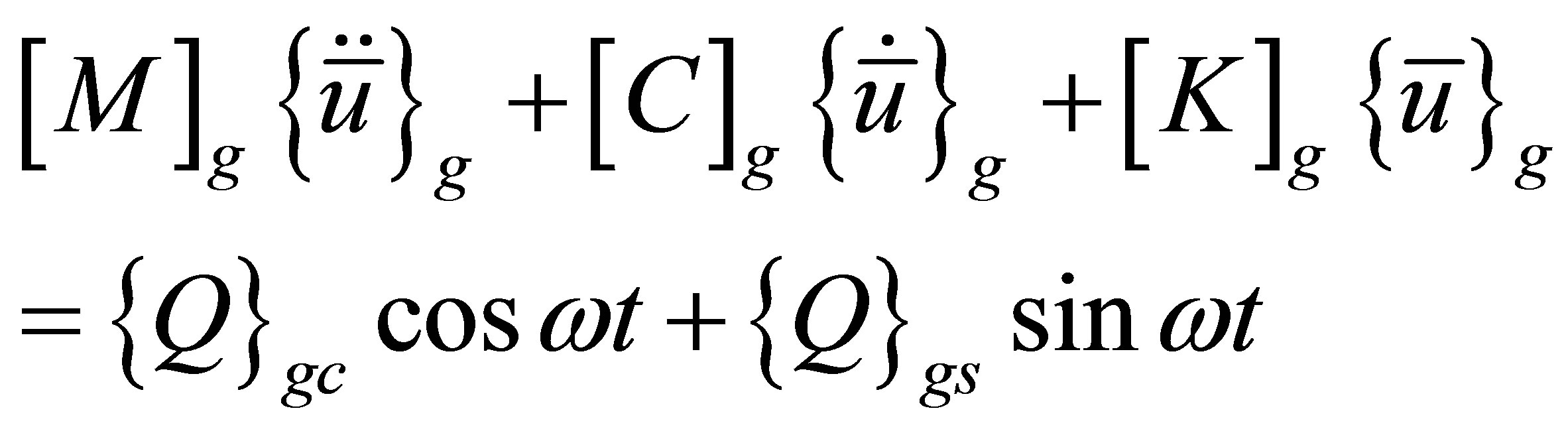 (27)
(27)
where,
2.6. Solution
To determine the steady-state propagation of a sinusoidal sound wave in the one-dimensional acoustic tube, we propose a solution in the following form
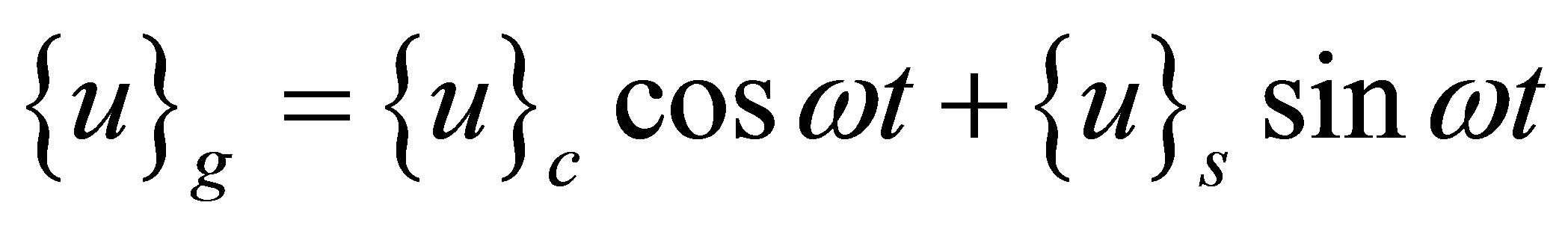 (28)
(28)
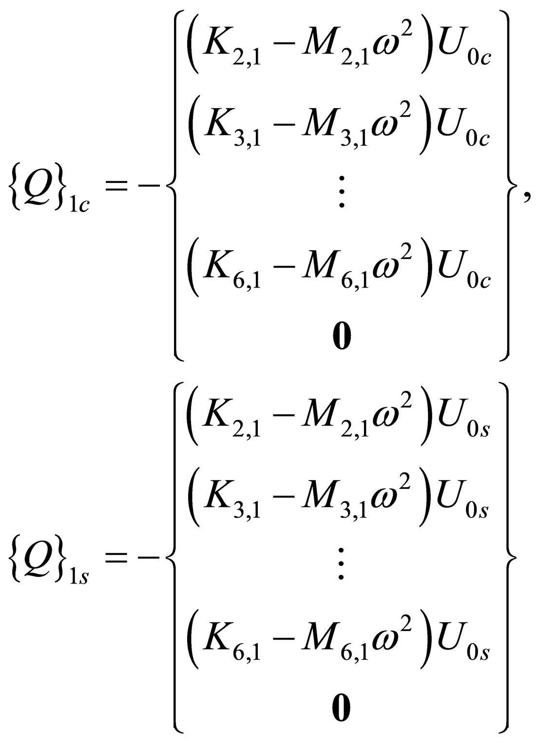
Substituting Equation (28) into Equation (27) and comparing the coefficients associated with sine and cosine harmonics, we arrive at the following equations
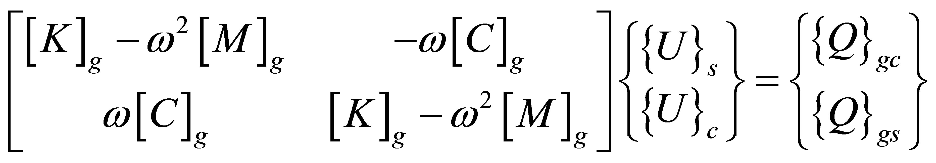 (29)
(29)
The above equations may be solved for the amplitudes of the nodal acoustic displacements and strains associated with the sine and cosine harmonics. To determine the acoustic pressure and acoustic velocity in medium k in the real domain, the following equations may be used
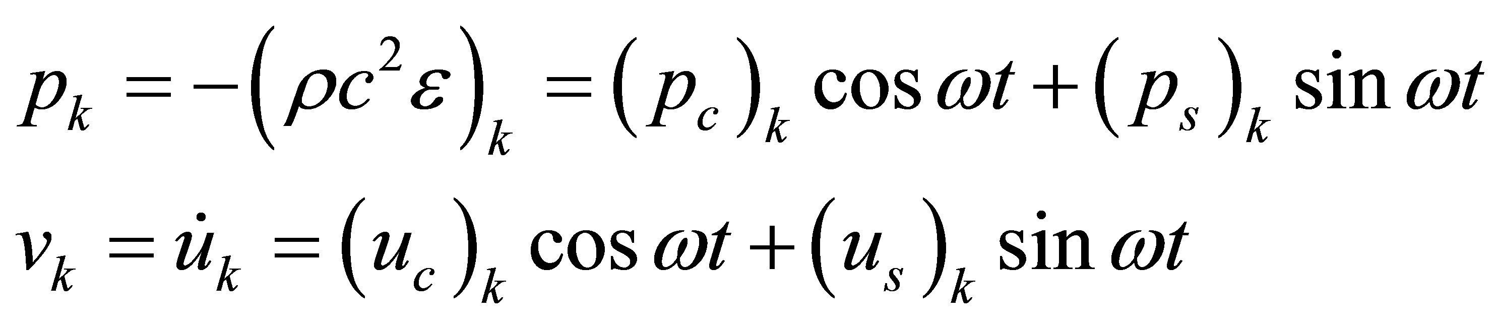 (30)
(30)
where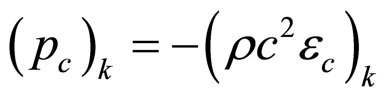 ,
, ; subscripts c and s represent cosine and sine harmonics of acoustic displacements, strains and pressures.
In studying steady-state acoustics, it is often desirable to represent the acoustic pressure in the complex domain, in which case the acoustic pressure is defined in the following manner
 (31)
(31)
It can be shown that the real and imaginary parts,  and
and , of the complex acoustic pressure
 , are related to the cosine and sine coefficients in Equation (30) by
Similar relationships may be written for other acoustic quantities, such as acoustic displacements and acoustic velocities.
3. Numerical Results
Before presenting numerical results for general applications, it is necessary to validate the methodology and the finite element procedure. This is done through two simple test cases, for which exact analytical solutions exist. For an acoustic system having three media (air, porous material and air), the topic of general interest, sound transmission loss, is investigated.
3.1. Sound Propagation in Air with Specified Acoustic Impedance
The first test case deals with sound produced by a vibrating piston for which  or
or , its propagation through a column of air, and its interaction with a solid medium characterized by a specified acoustic impedance, as shown in Figure 3(a). The specified acoustic impedance,
  , is defined as
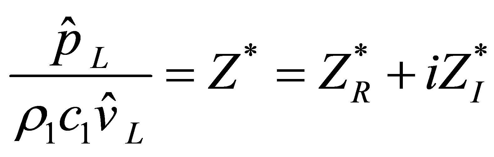 (33)
(33)
It can be shown that the exact analytical solution for the complex pressure everywhere may be written as
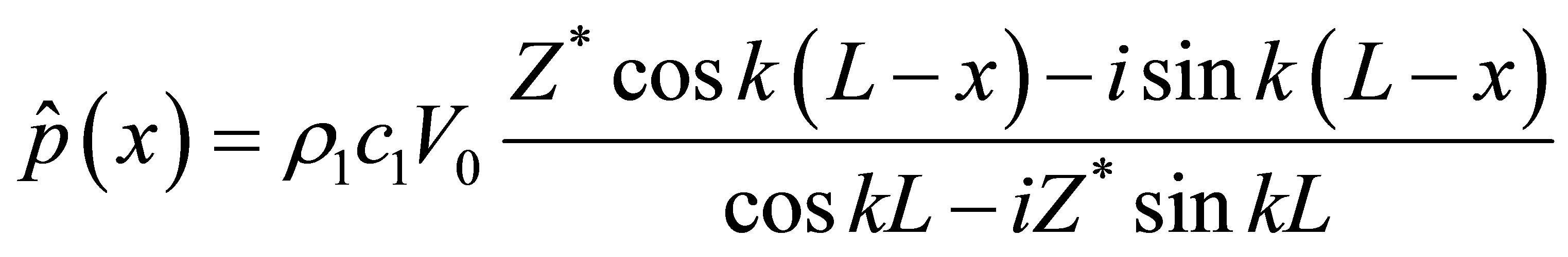 (34)
(34)
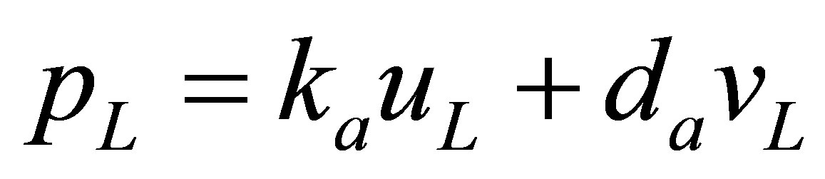
In the displacement-based model, the acoustic absorbing and reacting material with the specified impedance is equivalent to a massless piston subjected to the constraints of linear spring and viscous damping elements ( and
and ), as shown in Figure 3(b). From the equilibrium condition of the massless piston, the following relation may
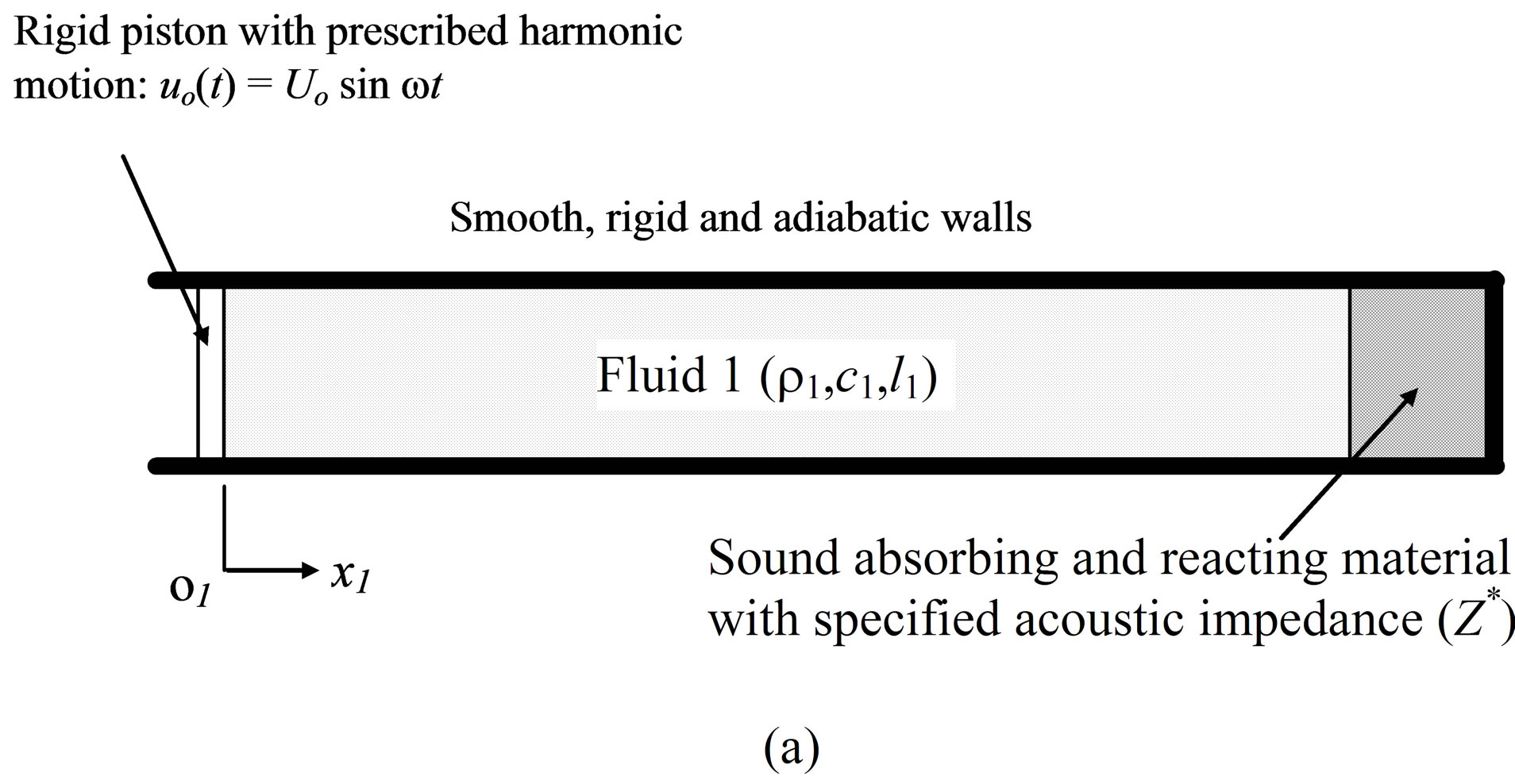
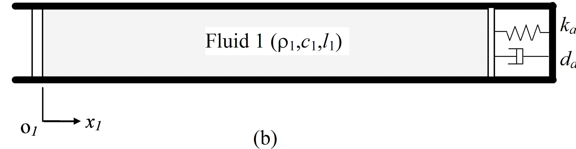
Figure 3. Test case 1: (a) a physical model of sound propagation in air and porous material with specified acoustic impedance; (b) an equivalent displacement-based model with porous material modeled as massless piston with spring and damping elements.
be obtained
 (35)
(35)
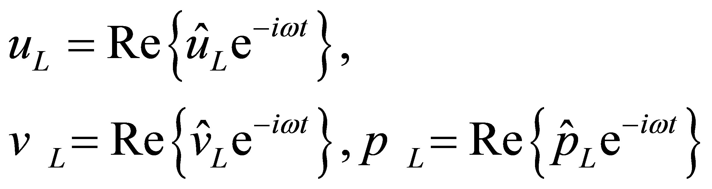
To determine the relationship between the acoustic impedance and values of  and
and , the following complex notations for steady state acoustic displacement, velocity and pressure at the air-solid interface are introduced
 (36)
(36)
where ,
,  and
and  are, respectively, the complex amplitudes of acoustic displacement, velocity and pressure at the interface.
Substituting Equation (36) into Equation (35), the equilibrium condition may be rewritten in terms of complex numbers as
 (37)
(37)
To derive the values of reactance and resistance coefficients from the real and imaginary parts of the specified acoustic impedance, the following relationship between complex velocity and complex displacement may be obtained from Equation (36)
 (38)
(38)
From Equation (37) and Equation (38), the following relationship may be obtained
 (39)
(39)
Comparing Equations (33) and (39), we may conclude that
 (40)
(40)
Numerical results were obtained using four finite elements and the analytical solution in Equation (34) for parameters given in Table 1. The real and imaginary acoustic pressures along the entire length of the air column are compared in Figure 4. It can be seen that the results from the finite element procedure are identical to the analytical solutions for both the real and imaginary acoustic pressures.
3.2. Sound Propagation in Air and Porous MateRial
The second test case, which was considered by Craggs [3], involves sound propagation in air and a porous material, as illustrated in Figure 5(a). The sound originates from a sinusoidally vibrating piston with varying amplitudes and frequencies. At the distant end of the porous material, the sound terminates. The equivalent properties of the porous material are calculated from the properties of standard air and three factors, as defined in Equation (18). In this test case, the structure factor and porosity factor are both taken to be one (Ks = 1, W = 1) and the resistivity (R) is allowed to vary. Values of other properties are given in Table 2. The absorption coefficients defined by Craggs [3] were calculated using four finite elements for the air and two finite elements for the porous material. The results are presented in Figure 5(b) for five values of resistivity and for excitation frequencies varying between 0 and 16 kHz. The computed sound absorption coefficients are identical to those reported by Craggs [3].
3.3. Sound Propagation in Air, Solid and Air
To study the sound transmission loss through a solid, an acoustic system having three components (air, solid and air), as depicted in Figure 1, is investigated. Since only the sound transmission loss as the sound propagates through the solid is of interest, the sound is assumed to be completely absorbed at some distance downstream from the solid material. This assumption ensures that the sound transmission loss calculations are not affected by sound reflected at the boundary of the system under consideration and the environment. The source of sound is again a vibrating piston whose frequency is allowed to vary over a wide range.
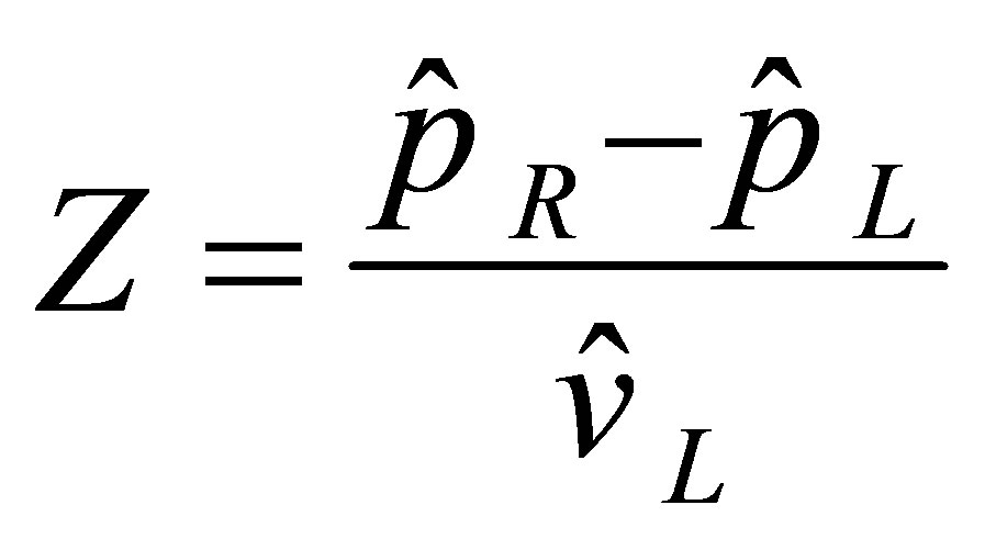
Under steady-state sound propagation conditions, the acoustic impedance, defined as the ratio of the complex acoustic pressure difference across the two surfaces of the solid (steel) to the input acoustic velocity, may be determined by
Table 1. Values of parameters used for test case 1.
Table 2. Values of Geometric and Material Properties Used for Test Case 2.
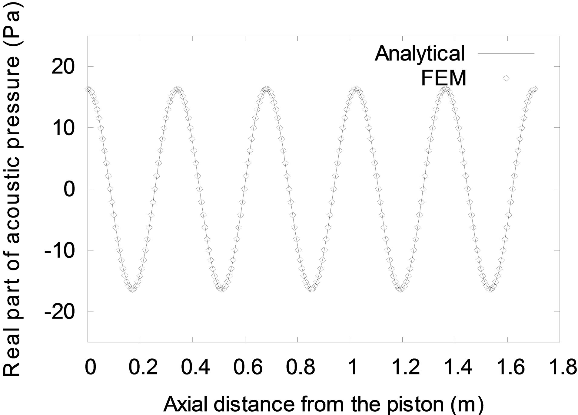
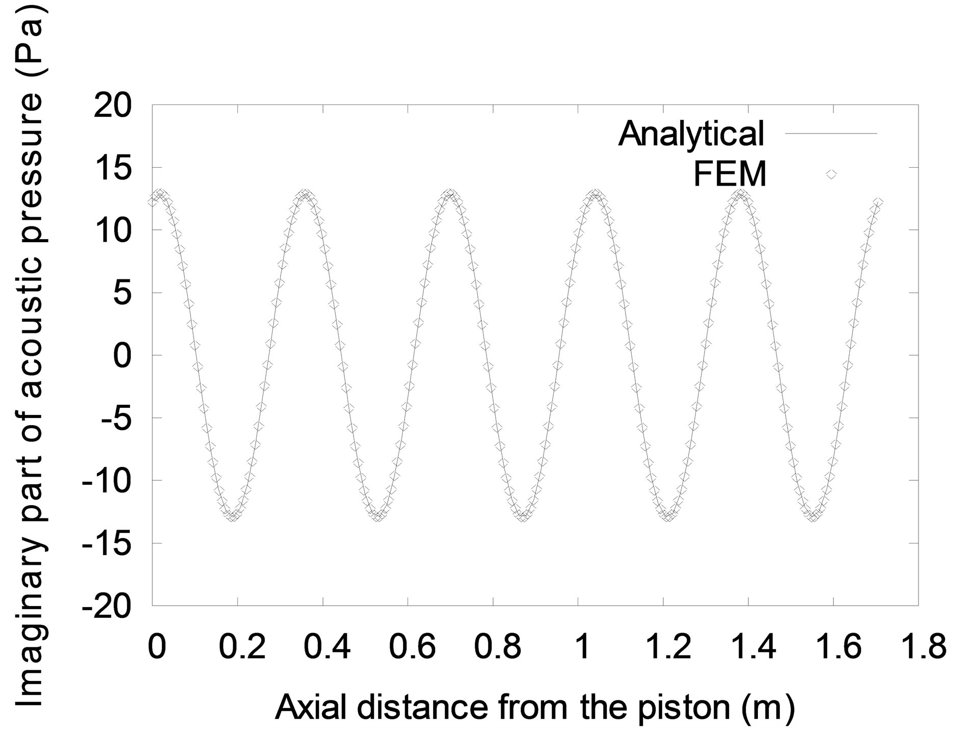
Figure 4. Steady state acoustic pressure for test case 1.
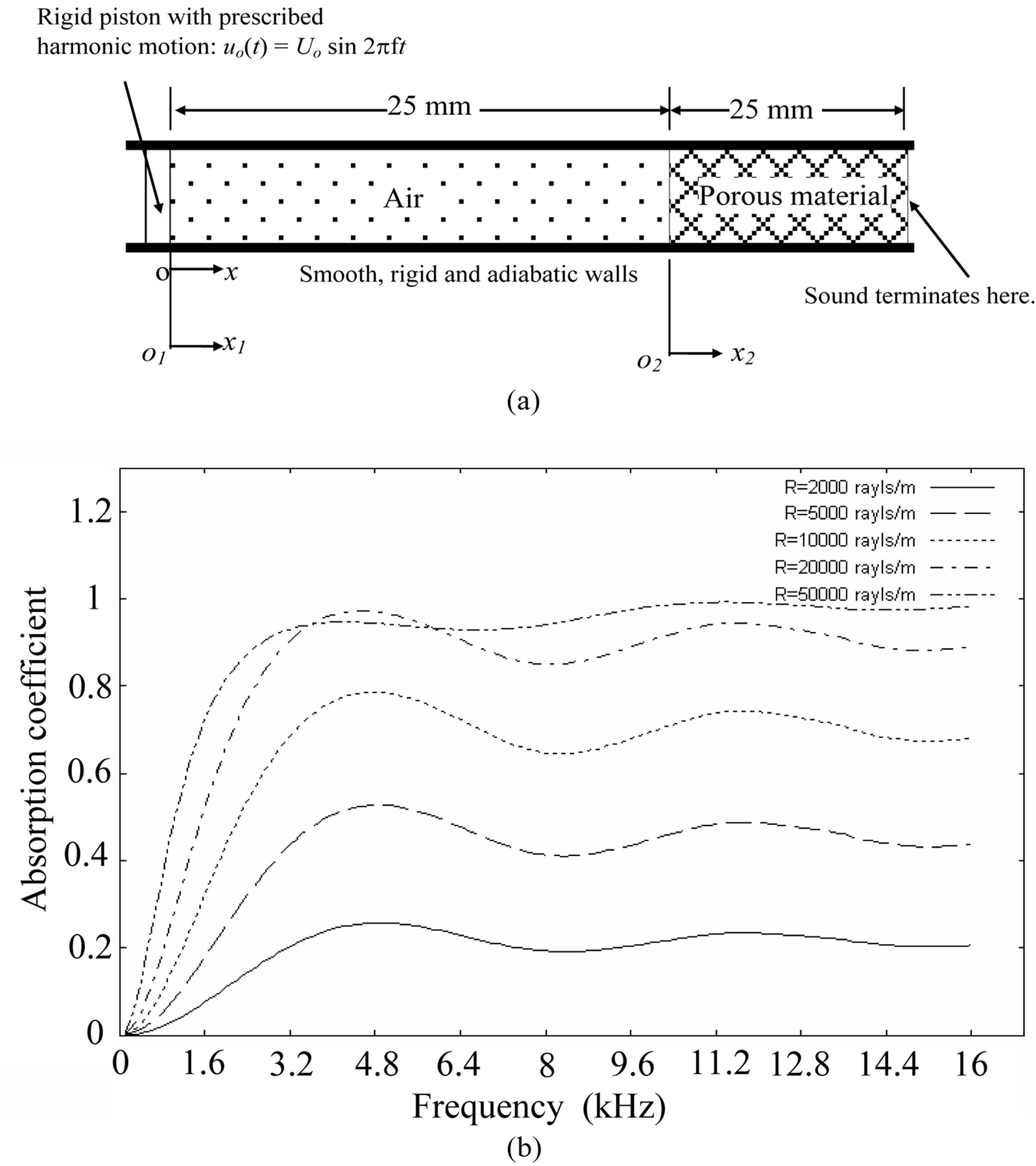
Figure 5. Test case 2: (a) a simple model used by Craggs [3], (b) computed sound absorption coefficient.
 (41)
(41)
where subscripts “L” and “R” represent the left and right surfaces of the solid. Equation (30) may be used to calculate the acoustic pressures on both sides of the solid and the incident velocity. Once the acoustic impedance is determined, the sound transmission loss across the porous material (in decibels) may be calculated using
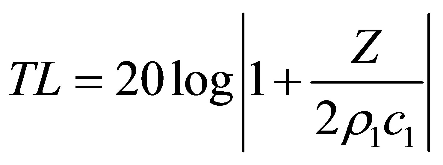 (42)
(42)
where  is the characteristic impedance of air.
Numerical results for sound transmission loss, obtained using the finite element method for a wide range of excitation frequencies, are presented in Figure 6 for a short solid and Figure 7 for a long solid. It can be seen that there is excellent agreement between the analytical solution and the finite element results for the sound transmission loss through solids of different lengths. The sound transmission loss increases linearly on the log-log scale with the frequency in accordance with the mass law or the limp wall model in the low frequency range, maintains a plateau value of just below 80 dB, and dips considerably at critical frequencies or natural frequencies of the solids.
4. Concluding Remarks
A finite element procedure is employed to investigate the
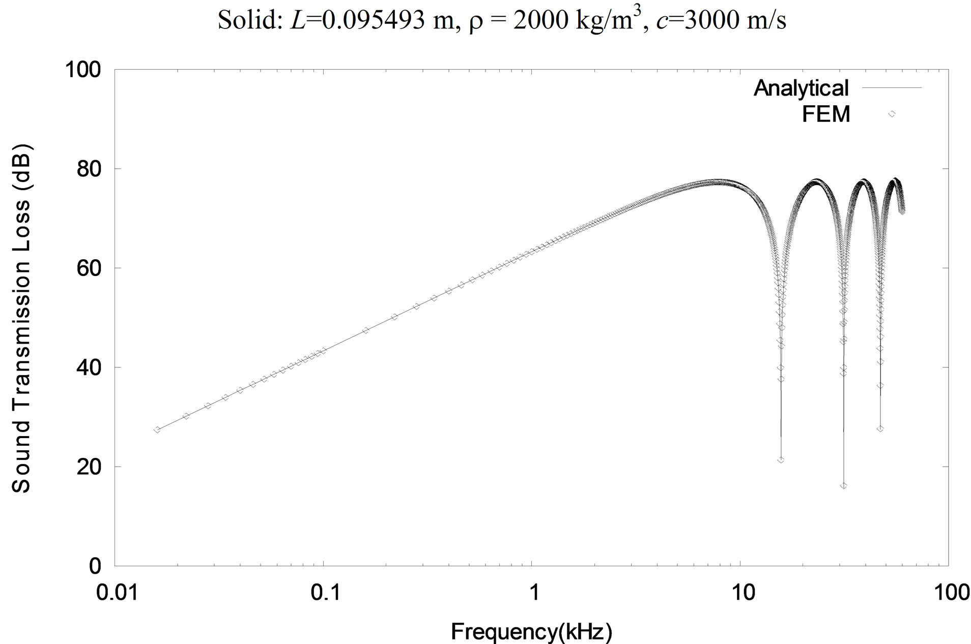
Figure 6. Sound transmission loss in a short solid.
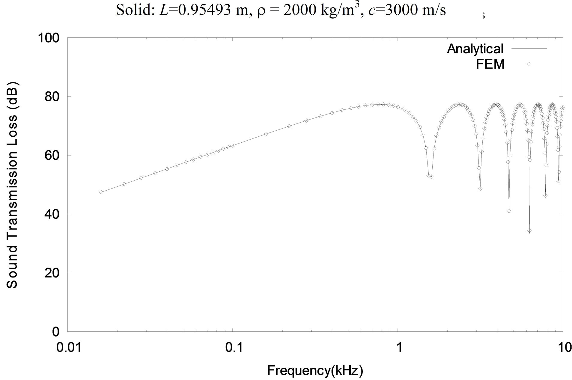
Figure 7. Sound transmission loss in a long solid.
sound transmission loss in various media. Numerical results, obtained using the proposed procedure, are in excellent agreement with the analytical solutions and independent solutions available in the literature.
REFERENCES
- G. M. L. Gladwell, “A Variational Formulation of Damped Acousto-Structural Vibration Problems,” Journal of Sound and Vibration, Vol. 4, 1966, pp. 172-186.
- A. Craggs, “A Finite Element Method for Damped Acoustic Systems: An Application to Evaluate the Performance of Reactive Mufflers,” Journal of Sound and Vibration, Vol. 48, No. 3, 1976, pp. 377-392.
- A. Craggs, “Coupling of Finite Element Acoustic Absorption Models,” Journal of Sound and Vibration, Vol. 66, No. 4, 1979, pp. 605-613.
- Y. J. Kang and J. S. Bolton, “Finite Element Modeling of Isotropic Elastic Porous Materials Coupled with Acoustical Finite Elements,” Journal of Acoustic Society of America, Vol. 98, No. 1, 1995, pp. 635-643.
- B. Tabarrok and F. P. J. Rimrott, “Variational Methods and Complementary Formulations in Dynamics,” Kluwer Academic Publishers, Kluwer, 1994.
- P. M. Morse and K. U. Ingard, “Theoretical Acoustics,” Elsevier, New York, 1968.
- A. Craggs, “A Finite Element Model for Rigid Porous Absorbing Materials,” Journal of Sound and Vibration, Vol. 61, No. 1, 1978, pp. 101-111.
- M. J. Crocker, “Handbook of Acoustics,” John Wiley & Sons, Inc., New York, 1998.
NOTES
*Corresponding author.