World Journal of Engineering and Technology
Vol.04 No.04(2016), Article ID:71401,10 pages
10.4236/wjet.2016.44052
On the Impact of the Frequency of Saved Thermal Time-Steps in a Weakly-Coupled FE Weld Simulation Model
Richard P. Turner, R. Mark Ward
PRISM2 Research Group, School of Metallurgy & Materials, The University of Birmingham, Edgbaston, Birmingham, UK

Copyright © 2016 by authors and Scientific Research Publishing Inc.
This work is licensed under the Creative Commons Attribution International License (CC BY 4.0).
http://creativecommons.org/licenses/by/4.0/


Received: June 20, 2016; Accepted: October 18, 2016; Published: October 21, 2016
ABSTRACT
Finite element (FE) modelling methods were implemented to perform a weakly- coupled weld simulation activity on a series of simple plate welds, to determine the effects of altering the frequency of saving the thermal time-step result upon the mechanical results. By definition, the thermal results will be unaffected, but the mechanical results are calculated from the saved thermal results, hence can be changed when the frequency of saving thermal time-steps is altered. By default, most weakly- coupled thermal-mechanical solvers will save every single thermal time-step, for accuracy. Results indicated that during the welding operation, the thermal time-steps could be reduced to saving 1-in-every-2 thermal time-steps with minimal loss in mechanical accuracy. However, during the cooling operation, every time-step was required to be saved. Whilst this seems almost counter-intuitive that the time-step during the cooling operation is in some way more critical than during welding, it must be stated that the FE software employed for this exercise has a setting allowing the time-steps to become progressively large during cooling, when thermal gradients are much lower and as such both thermal and mechanical calculations are easier to converge.
Keywords:
Fusion Weld, Simulation, Finite Element, Thermal, Mechanical, Distortion

1. Introduction
Weld simulation methods are becoming more widespread amongst both industrial and academic communities interested in weld research, due to their powerful results and the potential cost-savings associated with this tool [1] . Finite element (FE) analysis tools can be used to perform a weld simulation, and these types of models have been developed over a number of years. Several review papers of FE weld simulation methods and best-practice guides are available in the literature [1] - [4] , and successful weld simulation methodologies in a range of codes have been well-documented. Typically, most weld simulation methods consider simple plate-type geometry, for speed of calculation [5] . However, future modelling activities are more likely to be concerned with true component geometries, which could lead to much larger models, with a much- increased number of nodes and elements, and as such greatly increased solution-times [6] . In this work, the ESI Group FE software package Sysweld 2011 (and the pre- and post-processing add-on units in Visual Environment 7.5) has been used to perform the FE modelling work. The modelled geometry is limited to a simple bead-on-plate weld, for speed of calculation, with the plate used of dimensions; L = 150 mm, W = 100 mm, T = 5.5 mm in thickness.
FE models are typically performed either as a fully-coupled thermo-mechanical analysis, or a weakly-coupled thermal analysis followed by a mechanical analysis. The benefits of a fully-coupled thermo-mechanical analysis are that it accurately considers the heating arising from both an external heating source and heating by mechanical deformations induced in the part in the previous time-steps of its thermo-mechanical solution. However, in comparison to a weakly-coupled approach, this comes at the expense of greatly increased calculation times. For the modelling of certain welding processes― such as friction welding applications in which significant deformation produces a significant heating of the part-this type of modelling approach is necessary [7] . However, for fusion weld simulations, in which the resultant heating of the part due to the mechanical deformation occurring is negligible in comparison to the external heating source; a weakly-coupled analysis is commonly used as a modelling simplification [1] .
The mesh applied to the material splits up the continuum material into discrete finite elements, applicable for FE analysis to be applied. The size of the discrete elements used within the simulation will have an impact upon the solution-times, but also potentially the result. It is desirable to utilise the coarsest mesh-size possible which maintains a high level of accuracy―to enable accurate solutions to be calculated as fast as possible. Whilst literature has suggested the use of dynamic meshing [1] , which sees a finely meshed region “follow” the heat source, can be used for speed of calculation, for ease of set-up, the model here considers a static mesh, finely meshed along the weld line, with no re-meshing capabilities. Whilst the steep thermal gradients in the direction perpendicular to the direction of travel for the weld pool dictates that a very fine mesh is required, largely these gradients are not present in the direction of travel. The mesh employed in these models contained elements of size 2 mm in the welding direction, 0.6875 mm in the thickness (8 elements of even size over the thickness of 5.5 mm) and the mesh was graded in the direction perpendicular to the welding path, with smallest elements at the weld line measuring 0.2 mm, coarsening to the elements away from the weld line measuring 4 mm (see Figure 1).
In a weakly-coupled FE weld simulation using an appropriate software package, the

Figure 1. The meshing implemented in the plate weld FE models.
thermal analysis is initially calculated, and from these calculated thermal predictions the mechanical analysis is subsequently evaluated. The mechanical solution therefore is calculated from the thermal increments that have been saved to form the thermal result. Therefore, for a weakly-coupled analysis it has previously been considered necessary that every single calculated time-step of the thermal solution be saved, in order to predict as accurately as possible the resulting mechanical solution. This can lead to rather large thermal results files to be generated. However, the focus of the work will almost always be upon the mechanical results. Altering the frequency of saving the thermal time-step is a subtly different approach from altering the size of the time-step. If the size of the time-step was increased, this would produce a different thermal solution, with a reduced accuracy. Maintaining the same time-step size, but reducing the frequency that it is saved, maintains the accuracy of the thermal solution.
2. FE Modelling Work
A series of models was constructed, to consider a simple bead-on-plate weld geometry for a plate of dimensions; L = 150 mm, W = 100 mm, T = 5.5 mm in thickness, welded along a weld path running the length of the plate, at a constant weld speed. The models were analysed to determine how the mechanical results were affected when the frequency of the saved thermal time-steps is altered, becoming more coarse than the recommended default setting of saving every single increment. The models considered the same mesh, which can be seen in Figure 1.
The models considered a double ellipsoid function to describe the external heating source representing a typical TIG weld-pool. A double-ellipsoid, so-called Goldak function is used widely to represent the welding heat source for a variety of welding processes [8] [9] . The Goldak function is described by Equation (1):
 (1)
(1)
where q is the heat flux, Q is the power input (commonly Q = I×V), I is current, V is voltage, h the weld heat source efficiency, a, b and c are the depth, width and length semi-axes respectively of the melt pool, ν the weld travel speed, fi is the fraction of heat deposited in each of the front (ff) and rear (fr) halves of the pool, and x, y, z the local Cartesian co-ordinates. The model also considered a material definition suitable to describe the commonly used titanium alloy Ti-6Al-4V. Ti-6Al-4V is used for a variety of fusion welding applications, primarily within the aerospace sector, due to its excellent strength: density ratio. The time-step implemented in both the thermal and mechanical analyses of each model were of equal size?namely the time taken for the heating source to move 1 element along the weld path.
Additionally, once the welding process is completed, the model allows for a period of cooling, allowing the plates return to atmospheric temperature. By default, the FE model simulated using the Sysweld software has been used to attempt to perform the numerical calculations as fast as possible and as such allows the time-step to become very large during cooling, when there are greatly reduced computational difficulties within the model. Given that it is a TIG process being modelled, the boundary conditions used considered the process to occur in air. Any small effects upon cooling rate of the agitated argon gas shielding were ignored.
Initially, two models were built, one using the default setting of saving every single calculated thermal time-step, and one which saved only 1 in every 2 thermal time-steps. Clearly, this type of modelling set-up ensures that there are no effects upon the thermal results?simply “deleting” 1 in every 2 thermal time-steps has no impact at all upon the thermal results. However, there would be a knock-on effect upon the mechanical results. This is because in a weakly-coupled FE weld simulation, the mechanical results are computed from the saved thermal results. For any given time-step n, the mechanical solution at time-step n shall be calculated from the previous mechanical time-step n − 1, and the delta in the temperature field between the time-steps n-1 and n. Therefore, the mechanical solution for time-step n can be expressed as:
 (2)
(2)
where  and
and  are the calculated mechanical and thermal solutions respectively at any given time-step. Therefore, in changing the frequency of the saved thermal time-steps, the calculation for
  will consider a different
  solution. Clearly, as the model reduces the frequency of saved thermal time-steps, thus the solution will have to consider a larger jump in between successive time-steps in order to calculate
 . The distortions predicted on the right-side edge of the plate, at different stages through each of the two models, were considered.
A 3rd model was set-up, identical to model 2 (see Table 1), except for the frequency of thermal time-steps saved during the cooling period of the model, which was maintained as saving every time-step. As previously demonstrated, this modelling set-up has no change on the thermal results, but will have an impact upon the mechanical results. Again, the distortion at the right-side edge of the plate was considered for the two models. A final model (model 4) was set-up, this time with thermal time-steps during the welding period of the FE simulation saved at a frequency of 1-in-every-3, which would further reduce file size. As with model 3, the thermal calculations during cooling were saved at every single time-step. The resulting mechanical predictions were calculated, and again those results considering distortion in the z-axis were compared to model 1 (baseline) and model 3.
3. Results and Discussion
Evidence from FE modelling that the thermal solution is entirely unaffected by the procedure of changing the frequency of saving thermal time-steps is presented in Figure 2, where the two identical thermal fields at a particular stage throughout the welding and cooling process were calculated. This is because fundamentally the thermal

Figure 2. Thermal profiles taken during steady-state for (left) Weld Model 1, and (right) Weld Model 2. Note that the two profiles are identical, highlighting that changing the frequency of saving has no impact thermally.

Table 1. Matrix of weld simulation models.
calculations being performed are identical, except for the number of times the thermal results are saved as a transient file available to the subsequent mechanical calculation are different.
However, varying the frequency that thermal results are saved does have an impact upon the mechanical fields predicted by FE model. Thus the resulting mechanical solution for the two models (model 1 vs model 2) is presented displaying the distortion observed in the two models, at the instant the welding operation finishes (Figure 3(a)) and after the plate has cooled to room temperature (Figure 3(b)). Figure 4(a) & Figure 4(b) present a graphical representation of the distortions as predicted on the right-side edge of the plates as illustrated in Figure 3. It can be observed that the final distortion patterns predicted after the component cools for the two models are significantly different (Figure 4(b)). However, a comparison of these same distortion patterns at a time
 (a)
(a) (b)
(b)
Figure 3. (a) Distortion patterns at the instant the welding process finishes for: (left) Model 1 and (right) Model 2; (b) Distortion patterns after plates have cooled to room temperature for: (left) Model 1 and (right) Model 2.
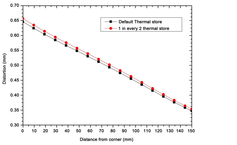 (a)
(a)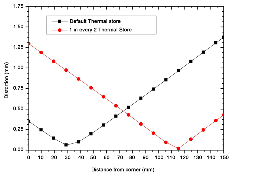 (b)
(b)
Figure 4. (a) Predicted distortion along right-hand edge at the end of the welding period, for Model 1―with default thermal time-step store; and Model 2―1-in-every 2 thermal time-step store; (b) Predicted distortion along right-hand edge, at the end of the cooling period, for Model 1―with default thermal time-step store; and Model 2―1-in-every 2 thermal time-step store.
just prior to the end of the welding stage of the model are remarkably similar (Figure 4(a)). This suggests that the procedure of changing the frequency of saving the thermal time-steps (from saving every time-step to saving 1-in-every-2 time-steps) has had little effect upon the mechanical results during the calculation of the welding process. It was only the change in frequency of saving thermal time-steps during cooling that had a significant effect upon mechanical predictions.
Figure 5(a) & Figure 5(b) display the final distortion pattern along the right-side edge of the plate for models 1 (baseline case) and 3. It can be observed that there is a good agreement between these final distortions, comparing the default (model 1) result with that from model 3; where a save of 1 in every 2 thermal time-steps is employed during the welding process, and a save of every thermal time-step is employed during the cooling process. This format of model set-up will clearly have a significant impact upon the thermal results file size for weld simulations with a very long welding path, virtually halving the space required to store these models; as in large industrial component weld simulations it is common for the welding process to occupy 90% - 95% of the time-steps within the simulation, and cooling only occupying 5% - 10% of the used time-steps.
Figure 5(c) shows the predicted distortion on the plate in model 4. Comparing to Figure 5(a) and Figure 5(b), a significant impact upon the final distortion of the whole plate has been obtained by reducing the frequency of saving thermal time-steps during the welding period of the model to 1-in-3. Again, the results were interrogated by plotting the distortion at the right-side edge of the plate. This is presented in Figure 6. The results presented demonstrate that the accuracy of the final distortion calculations decreases significantly when only 1 in 3 thermal time-steps are saved during the welding operation. This would strongly suggest that as the iterative solver is now being forced to use saved thermal time-step results from further back in its new mechanical calculation, so interpolation errors have been growing to produce a considerable loss of accuracy in the calculated mechanical results.
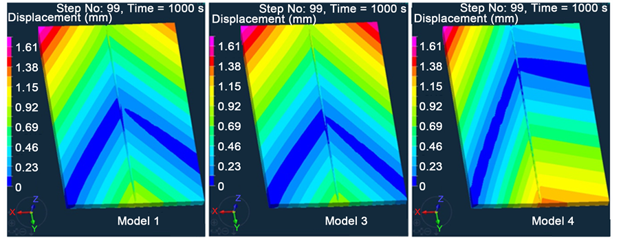 (a) (b) (c)
Figure 5. Distortion patterns after plates have cooled to room temperature for: (left) Model 1 (centre) Model 3, and (right) Model 4.
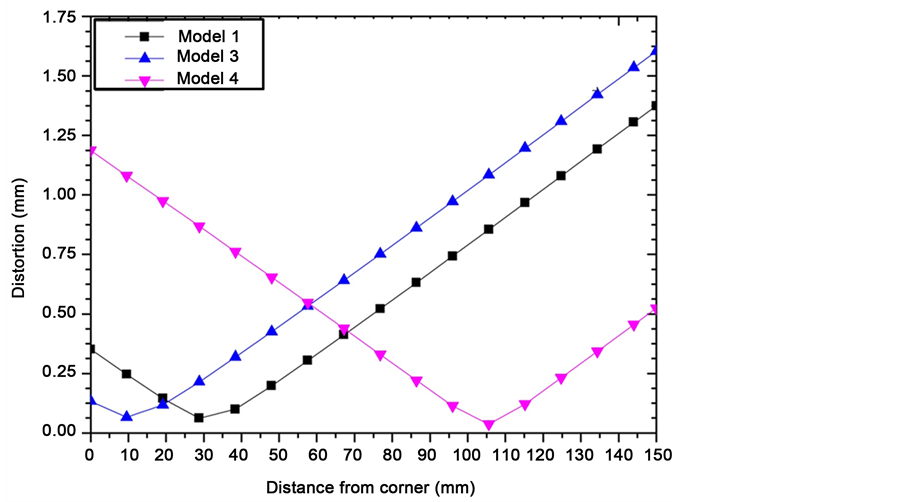
Figure 6. Predicted distortion along right-hand edge, taken after plate has cooled to room temperature for: Model 1, Model 3 and Model 4.
4. Conclusions
A series of 4 FE models have been created and run, to investigate the impact that altering the frequency of saving thermal time-steps has upon the mechanical results of these simulations. The following conclusions have been drawn:
1) The frequency of saving the thermal time-step results in an FE weld simulation, during the actual welding time, can be reduced from every step to 1 step in every 2 with only a small decrease in the modelling accuracy. However, any further reduction in thermal time-step save leads to incorrect trends being predicted by the FE model.
2) Time-step requirements during the cooling process after welding are more complicated than initially assumed. In the case of a Sysweld model, where the solver attempts to make the time-step size during cooling to be as large as possible, the frequency of saved results for the thermal time-step must be maintained as every single time-step in order for the mechanical solution to maintain accuracy. This suggests that the cooling process following a welding operation is very important to be fully understood, for any weld simulation activity to be successful in accurately predicting weld-induced distortions.
3) The resulting trends observed from of these FE predictions could have a significant impact. By following the recommendations here, an FE computational engineer working upon the simulation of a welding process could optimise the solution in terms of reducing the calculation time taken (by reducing the computational read/ write requirements) and reducing the disk-space taken up by the calculated results file, two issues often faced by FE computational engineers.
Acknowledgements
The work was undertaken as part of the COMSTAR project, funded by Advantage West Midlands (AWM), a collaborative project between the University of Birmingham, Rolls- Royce plc and ESI Group. The author would like to thank colleagues at the PRISM2 research group in Metallurgy & Materials at the University of Birmingham for support and advice during this investigation. Thanks are offered to Rob Uings of ESI Group (at that time) for technical support with the software Sysweld and the pre- and post- processing unit Visual Environment.
Cite this paper
Turner, R.P. and Ward, R.M. (2016) On the Impact of the Frequency of Saved Thermal Time-Steps in a Weakly-Coupled FE Weld Simulation Model. World Journal of Engineering and Technology, 4, 528-537. http://dx.doi.org/10.4236/wjet.2016.44052
References
- 1. Lindgren, L.E. (2006) Numerical Modelling of Welding. Computer Methods in Applied Mechanics and Engineering, 195, 6710-6736.
http://dx.doi.org/10.1016/j.cma.2005.08.018 - 2. Lindgren, L.E. (2001) Finite Element Modelling and Simulation of Welding, Part 1— Increased Complexity. Journal of Thermal Stresses, 24, 141-192.
http://dx.doi.org/10.1080/01495730150500442 - 3. Lindgren, L.E. (2001) Finite Element Modelling and Simulation of Welding, Part 2— Improved Material Modelling. Journal of Thermal Stresses, 24, 195-231.
http://dx.doi.org/10.1080/014957301300006380 - 4. Lindgren, L.E. (2001) Finite Element Modelling and Simulation of Welding, Part 3— Efficiency and integration. Journal of Thermal Stresses, 24, 305-334.
http://dx.doi.org/10.1080/01495730151078117 - 5. Stone, H.J., Roberts, S.M. and Reed, R.C. (2000) A Process Model for the Distortion Induced by the Electron-Beam Welding of a Nickel-Based Superalloy. Metallurgical Transactions A, 31, 2261-2273.
http://dx.doi.org/10.1007/s11661-000-0143-x - 6. Turner, R., Huang, J., Gebelin, J., Ward, R.M. and Reed, R.C. (2012) Modelling of the Electron Beam Welding of a Titanium Aeroengine Compressor Disc. 9th Trends in Welding Research, Chicago, June 2012.
- 7. Turner, R., Gebelin, J., Ward, R.M. and Reed, R.C. (2011) Linear Friction Welding of Ti-6Al-4V: Modelling and Validation. Acta Materialia, 59, 3792-3803.
http://dx.doi.org/10.1016/j.actamat.2011.02.028 - 8. Goldak, J., Chakravarti, A. and Bibby, M. (1984) A New Finite Element Model for Welding Heat Sources. Metallurgical Transactions B, 15B, 299-305.
http://dx.doi.org/10.1007/BF02667333 - 9. De, A., Maiti, S.K., Walsh, C.A. and Bhadeshia, H.K.D.H. (2003) Finite Element Simulation of Laser Spot Welding. Science and Technology of Welding and Joining, 8, 377-384.