Journal of Mathematical Finance
Vol.08 No.03(2018), Article ID:86504,14 pages
10.4236/jmf.2018.83034
A Method for Portfolio Selection Based on Joint Probability of Co-Movement of Multi-Assets
Tianmin Zhou
School of Systems Science, Beijing Normal University, Beijing, China

Copyright © 2018 by author and Scientific Research Publishing Inc.
This work is licensed under the Creative Commons Attribution International License (CC BY 4.0).
http://creativecommons.org/licenses/by/4.0/


Received: July 6, 2018; Accepted: August 4, 2018; Published: August 7, 2018
ABSTRACT
This paper presents a method of portfolio selection for reducing co-related risks. Differing from the Markowitz’s mean-variance framework, we use the joint probability of co-movement of multi-assets (JPCM) as a measure of risks, and under the condition of minimizing the JPCM, we pinpoint the optimal portfolio by optimizing the JPCM matrix of paired assets. At the same time, we use the shape parameter of generalized error distribution (GED) to measure the tail shapes of different portfolios. The empirical results for China’s stock market show that the JPCM portfolios significantly outperform naive-diversified portfolios (1/N-rule) and minimum-variance (MV) in terms of the tail shape of portfolio distribution.
Keywords:
Portfolio Selection, Mean-Variance, Joint Probability Density, Cross-Entropy Approach

1. Introduction
Portfolio selection and optimization has been a fundamental problem in finance ever since Markowitz laid down the ground-breaking work that formed the foundation of what is now popularly known as Modern Portfolio Theory [1] . The main idea of MPT is “never putting all your eggs in one basket”. Markowitz posed the mean-variance analysis by solving a quadratic optimization problem. This approach has had a profound impact on the financial economics and is a milestone of modern finance. However, there are documented facts that the Markowitz portfolio is very sensitive to errors in the estimates of the inputs. Namely, the allocation vector that we get based on the empirical data can be very different from the allocation vector we want based on the theoretical inputs [2] . Hence, the mean-variance optimal portfolio does not perform well in empirical applications, and it is very important to find a robust portfolio that does not depend on the aggregation of estimation errors.
Various efforts have been made to modify the Markowitz unconstrained mean-variance optimization problem to make the resulting allocation depend less sensitively on the input vectors, such as the expected returns and covariance matrices. Black and Litterman showed that although the covariances of a few assets can be adequately estimated, it is difficult to come up with reasonable estimates of expected returns [3] . They proposed that expected excess returns for all assets can be obtained by combining investor views with market equilibrium. Roon, Nijman and Werker considered testing variance spanning with the no-short-sale constraint [4] . Goldfarb and Iyengar studied some robust portfolio selection problems that make allocation vectors less sensitive to the input vectors [5] . The seminal paper by Jagannathan and Ma imposed the no-short-sale constraint on the Markowitz mean-variance optimization problem and gave insightful explanation and demonstration of why the constraints help even when they are wrong [6] . They demonstrated that their constrained efficient portfolio problem is equivalent to the Markowitz problem with covariance estimated by the maximum likelihood estimate with the same constraint. However, as demonstrated in this paper, the optimal no-short-sale portfolio is not diversified enough. The constraint on gross exposure needs relaxing in order to enlarge the pools of admissible portfolios. Fan, Zhang and Yu showed that the gross-exposure constrained by mean-variance portfolio selection has similar performance to the optimal theoretical portfolios with no error accumulation effect and no-short-sale portfolio is not diversified enough and can be improved by allowing some short positions [7] . Colon adopted an A-DCC volatility model to generate the covariance forecasts in order to adjust to prevailing risk environments [8] . Bessler, Opfer and Wolff paid attention to the performance of the Black and Litterman model, and found that the BL model significantly outperforms naive-diversified portfolios, mean-variance, Bayes-Stein, and minimum-variance strategies in terms of Sharp ratios [9] . Becker, Gürtler and Hibbeln compared the performance of traditional mean-variance optimization with Michaud’s re-sampled efficiency in a large number of relevant estimators and found that Michaud outperforms Markowitz when the variance of estimators is large [10] . Pfiffelmann, Roger and Bourachnikova compared the asset allocations generated by BPT (Behavioral Portfolio Theory) and MPT without restrictions [11] , and showed that the BPT optimal portfolio is Mean Variance (MV) method efficient in more than 70% of cases.
These excellent works above just consider how to reduce the volatility in the financial markets. However, investors are more concerned about co-related risk of the portfolio returns, namely the possibility of huge losses in a portfolio. In the stock market, if the log-returns of two stocks are norm distributions, correlation coefficient can depict the relationship between two stocks and covariance is a good risk measure of two stocks. However, in the case of non-normal distribution, covariance is not able to accurately measure the risk between two stocks. Instead of the covariance, we use the joint probability of co-movement of two stocks to measure the co-related risks of portfolios. The co-movement of two stocks represents that the returns of two stocks simultaneously exceed the given threshold (superior and inferior threshold). We use revised multidimensional normal distribution of log-return of multi-assets to calculate the probability. With the criterion of minimizing the joint probability of co-movement of two stocks, we obtain the portfolio with the smallest co-related risks by optimization procedure. This method overcomes the shortcoming of covariance that merely measures risks of portfolio from a linear relationship.
The remainder of the article is organized as follows: we start with a short description of the MV approach and JPCM approach in Sections 2. In Section 3, we explain the database and present the empirical results. Our findings are summarized in Section 4.
2. Portfolio Optimization Methodology
2.1. Markowitz Mean-Variance Optimization
Markowitz built his portfolio selection contributions to MPT on the following key assumptions:
• All investments are completely separable, and each investor can select as much or as little investments as they wish (have ability to spend).
• Investors are willing to select portfolios only depending on expected value and variance (standard deviation) of portfolio returns.
• Investors know in advance the return distribution which satisfies the normal distribution.
• Investors follow these basic rules when they choose a portfolio: 1) They seek to maximize returns while minimizing risk. 2) They are only willing to accept higher amounts of risk if they are compensated by higher expected returns.
According to the above assumptions, Markowitz put forward the method of computation for expected return and variance of a portfolio and established the Efficient Frontier Theory and Mean-Variance optimization:
(1)
where represents the vector of portfolio shares of the p risky assets, is the sample expected returns, is a given return, the sample variance-covariance matrix, in none existence of short-sale market, .
2.2. Joint Probability of Co-Movement of Multi-Asset
In the stock market, the loss distribution of stock returns reflects stock risks and this distribution can provide the risk criterion for the stockbroker in the investment decisions; therefore, the accurate measurement risk is a key factor in the risk management. When stockbrokers want to invest multi-asset, only considering a single distribution is difficult to describe the relationships between multi-assets.
On condition that price process is geometric Brownian motion, the dependence between log-return of two assets can be described as follows: Let price of two dependence assets be , and their price process be
and
where and is the correlation coefficient. During a continuous-time model, log-return of two assets are and , then and . The correlation coefficient between two assets can be obtained by calculating .
In the real market, if the correlation between two assets is linear and the log-returns are normal distribution, we can easily compute and make a perfect allocation for assets. However, the reality of discovery is a different matter that the asset returns may represent peak and heavy-tailed features and the original method above cannot describe the relationship between assets precisely, for example, how to find the nonlinear function in and how to confirm the distribution of returns if we do not know the price process.
The clustering of large moves and small moves in the price process is one of the most important features of the volatility process of asset prices. Mandelbrot [12] and Fama [13] both reported evidence that large changes in the price of an asset are often followed by other large changes, and small changes are often followed by small changes. This evidence leads to the extreme risks often associated with excess returns. We should use the joint probability of co-movement of multi-asset to describe this joint effect. As noted by Segoviano [14] , we define the joint probability of co-movement of assets returns as follows:
(2)
where and represent threshold values, represents the joint distribution of multi-variate in portfolio, and Equation (2) represents the probability of p assets with returns co-moving to both maximum and minimum value during some period.
Considering how to get the joint probability density of multivariate in a portfolio, the traditional route is to impose parametric distributional assumptions, for example, the most common parametric distributions are the conditional normal distribution, the t-distribution and the mixture of normal distributions. However, in fact, we can only establish the model through finite information, which will inevitably lead to errors in estimating parameters. Therefore, rather than imposing parametric distributional assumptions, we using the Minimum Cross Entropy Distribution proposed by Kullback [15] and Good [16] embedded in our model.
For p assets , their price logarithmic returns are , and the cross-entropy objective function is defined as follows:
(3)
where is the multi-variates prior distribution, and the posterior distribution is .
Then we assume that the multi-variate prior distribution is p-dimensional joint normal distribution, i.e. , is the mean vector, and is the variance-covariance matrix. Our objective is to minimize the cross entropy distance between the posterior and the prior , and the posterior one need to satisfy the constraints as follows:
(4)
(5)
(6)
where and is the threshold which represents risk occur when returns of an asset are below it, is the threshold which represents excess occur when returns of an asset are beyond it, is the risk aversion coefficient, is the prior inverse CDF of the marginal distribution of asset logarithmic returns, and are the empirically observed probabilities of extreme value for each asset in the portfolio. and represent indicating function as follows:
Next, we minimize the Equation (3) by Lagrange multipliers and let
where , ,
, , and D is a p-dimensional
space satisfying , minimizes the cost functional above
at the boundary planar L of the p-dimensional D, and , where is a given fully small positive, and is an any function of satisfying , that is . The optimization procedure can be performed by computing the following variation:
namely,
where , and then . Due to the any function , and we can get
that is,
,
and the optimal solution is represented by the following multivariate density as:
(8)
where and are the correction factors to the prior density. We can obtain these factors by solving the Equations (4), (5) and (6) and the co-movement among p assets is
(9)
2.3. JPCM Optimization
For p assets, the weight of each asset is expressed as and weights should be . During a period of time T, we let be the random vector of p assets price logarithmic returns, and observe it every minute and obtain a total n observations. First, we specify the distribution of the logarithmic returns of the p assets as a joint normal distribution. If the hypothesis that the return series of multi-assets obey joint normal distribution is true, we can easily find a best w to minimize the risk of . However, the relationships between assets are nonlinear and return series has peak and heavy-tailed features in real market. The covariance between assets is not a very good measure for relationships. So we use JPCM method to establish the relationships between two assets and we specify the prior distribution of two assets as
(10)
where is bivariate function, and , , is the covariance matrix.
Then, we obtain the empirically observed probabilities of the threshold value according to the actual data: and . Therefore,
the posterior PDF of paired assets and
are obtained, according to the Equation (9) and the corresponding JPCM matrix is
(11)
Then in none existence of short-sale market, and we establish quadratic program with JPCM matrix as follows:
(12)
where represents the vector of portfolio shares of the p risky assets, is the sample expected returns, is a given return, , in none existence of short-sale market, .
3. Empirical Analysis
3.1. Data
This paper selects the SSE (Shanghai Stock Exchange) 50 constituent stocks as empirical data which are composed of 50 large-cap stocks. We randomly selected 10 stocks as a portfolio with replacement method, finally, collected 100 samples.
The trading day of each stock was selected from 2015-01-05 to 2015-11-2, a total of 201 trading days. In this period, China’s stock market experienced the formation from the bull market with almost all stock prices jumped up to the stock market crash with nearly all liquidity completely lost, which has certain representation of mechanism transformation in stock market.
Then, data cleaning of sample stocks is based on the following principles. First, we computed the trading hours of ten stocks in each day, and eliminated the intraday trading data in ten stocks if the trading hours were less than 2 hours. Second, we took the intersection of trading dates of ten stocks in order to ensure the uniform trading date. Third, we took the intersection of one-minute price data of ten stocks in each day. Fourth, as noted by Andersen [17] , five-minute sampling frequency in stock prices has contributed to reducing price noise, so we use a five-minute return horizon as the effective time record.
3.2. Optimization Results
201 trading days is divided into two periods. The first period from 2015-01-05 to 2015-06-09 has main characteristics that almost all stock prices jumped up, and the second period from 2015-06-10 to 2015-11-02 that almost all stock prices plummeted. We apply JPCM method, Markowitz model and 1/N-rule during two periods to optimize portfolios.
When optimizing JPCM matrix during two periods, we set the same risk aversion coefficient to 0.001 , then calculated the JPCM matrix, finally optimized the weight of portfolios according to Equation (12). Meanwhile, we set 10 assets weights equal to 1/10, and under the same conditions (we establish quadratic program without return constrain) used quadratic programming method to optimize Markowitz’s Mean-Variance model. The weights of three methods were obtained respectively, shown in Figure 1.
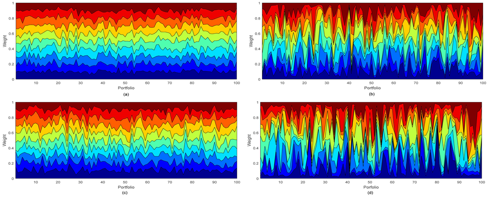
Figure 1. JPCM and MV optimized portfolio weights. This figure describes the JPCM and MV optimized portfolio weights for 100 during two periods. Subplots (a) and (b) represent the JPCM weights and MV weights respectively during first period. Subplots (c) and (d) represent the JPCM weights and MV weights respectively during second period. The horizontal axis of this chart is portfolios and the vertical axis is weights. The regions with similar color represent the same series assets in 100 samples. Seen from the chart, the variation of MV weights between two periods is bigger than that of JPCM weights. (a) CM optimized portfolio weights during first period; (b) MV optimized portfolio weights during first period; (a) CM optimized portfolio weights during second period; (a) MV optimized portfolio weights during second period.
3.3. Use Tail Shape Index to Measure Portfolio Risk
The probability of extreme events of the portfolio can be described by the generalized error distribution. This is because the tail shape index of the generalized error distribution can calculate a tail thickness of a distribution accurately. General error distribution (GED) has been widely used in modeling volatility of high-frequency time series with heavy tail. The probability density function (pdf) of the standardized GED is given by:
(13)
For s > 0 and , where and denotes the Gamma function. Nelson pointed that the GED reduces to the standard normal distribution when s = 2, and s represents the tail thickness parameter, i.e., for the tail of the GED is thicker than that of the normal distribution, and the GED has a thinner tail for s > 2 [18] . We calculate the tail thickness parameter of portfolios respectively during both period, as shown in Table 1.
From Table 2, we can conclude that the tail shape index of JPCM portfolio is greater than 1/N rule portfolio and Markowitz portfolio. Meanwhile, we also find that there is the asymmetry of tail indices during different period, i.e. the tail shape index of stock return is greater when in the bull market than in bear market, which represents that probability of risk is increased when a stock falls.
Then we show two figures about the distribution of return between three methods. Because of the space limitations, we select representative figures in our empirical results. We use the log-return of twentieth portfolios optimized by three methods as data and plot figures by fitting the distributions of these portfolios. The subplots inserted in figures are the photomicrographs of tail distribution. Although the tail distribution of JPCM model is thinner than other methods, it is difficult to tell the difference by naked eye. In Figure 2, the tail shape

Table 1. Tail thickness parameters of different methods.
This table reports the tail indices of portfolios return distributions during two periods, where s11, s12, s13 in first period separately represent the indices of JPCM portfolio, Markowitz portfolio and 1/N rule portfolio from 2015-01-05 to 2015-06-09 and s21, s22, s23in second period separately represent the indices of JPCM portfolio, Markowitz portfolio and 1/N rule portfolio from 2015-06-10 to 2015-11-02.
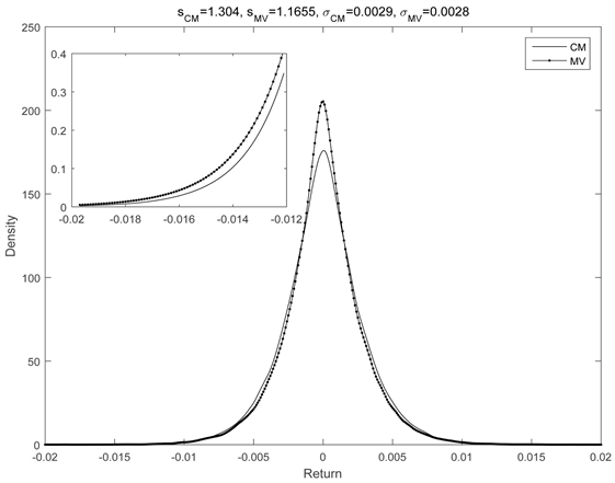
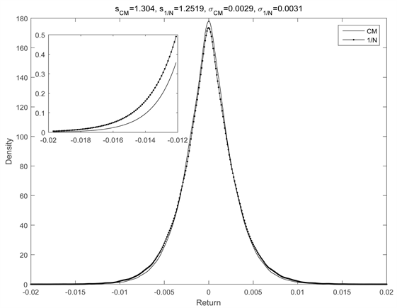
Figure 2. The distribution comparison between JPCM, MV and 1/N.
Table 2. Mean value of return in different methods.
This table reports mean value of return during two periods, where m11, m12, m13 in first period separately represent mean value of return in JPCM portfolio, Markowitz portfolio and 1/N rule portfolio from 2015-01-05 to 2015-06-09 and m21, m22, m23 in second period separately represent the mean value of return in JPCM portfolio, Markowitz portfolio and 1/N rule portfolio from 2015-06-10 to 2015-11-02.
index of JPCM portfolio is 1.304, the tail shape index of MV is 1.1655 and the tail shape index of 1/N is 1.2519. We can find that JPCM portfolio has thinnest tail shape.
In order to compare the difference in the tail indices of these portfolios optimized by different methods, we carry out a paired-samples t-test method to analyze every discrimination of the tail indices. Paired-samples t-test substantially is used for determining whether there is a systematic deviation between paired test data, i.e. the difference between paired data can be seen as a sample of a normal distribution, and infer whether there is a significant difference between co-related risks of these portfolios optimized by different methods through two-sided test on the zero mean.
Therefore, these tail indices during two periods are used to establish a paired sample as follows: {s11-s12, s11-s13, s12-s13}, {s21-s22, s21-s23, s22-s23} and we analyze these data with paired-samples t-test with the results shown in Table 3 and Table 4.
Table 4 reports the results of paired-sample t-test for different optimization methods during first period. We find that: 1) There exist significant differences between the tail shape index of JPCM portfolio and of 1/N rule portfolio, and JPCM portfolio has a significantly higher tail shape index to 1/N rule, i.e. JPCM portfolio has a thinner tail than 1/N rule. 2) There exist significant differences between the tail shape index of JPCM portfolio and of Markowitz portfolio, and JPCM portfolio has a significantly higher tail shape index to Markowitz, i.e. JPCM portfolio has a thinner tail. 3) There exist significant differences between the tail shape index of 1/N rule portfolio and of Markowitz portfolio, and 1/N rule portfolio has a significantly higher tail shape index to Markowitz. Recently, 1/rule model performs better than MV (Minimum-Variance) model in research community, when optimizing in high-dimension space. Text heads organize the.
The table reports the results of paired-sample t-test for different optimization methods during second period. We find that: 1) There exist significant differences between the tail shape index of JPCM portfolio and of 1/N rule portfolio,
Table 3. Paired-sample t-test during first period.
Table 4. Paired-sample t-test during second period.
and JPCM portfolio has a significantly higher tail shape index to 1/N rule, i.e. JPCM portfolio has a thinner tail than 1/N rule. 2) There exist significant differences between the tail shape index of JPCM portfolio and of Markowitz portfolio, and JPCM portfolio has a significantly higher tail shape index to Markowitz, i.e. JPCM portfolio has a thinner tail. 3) There exist significant differences between the tail shape index of 1/N rule portfolio and of Markowitz portfolio, and 1/N rule portfolio has a significantly higher tail shape index to Markowitz.
The results above show that: 1) the distribution of JPCM portfolio has a significantly higher tail shape index (a higher tail shape index represents a thinner tail) than that of naive-diversified portfolio and Markowitz portfolio, whether we optimize these portfolios from 2015-01-05 to 2015-06-09 or from 2015-06-10 to 2015-11-02, i.e., extreme value occurs with small probability in JPCM portfolio, which represents that this method can reduce risk of portfolio significantly. 2) Tail shape index has obvious asymmetry in both periods, i.e., tail indices of portfolios optimized by three methods in first period are larger than that in second period, which means that the tail shape index of a portfolio when its price rising is greater than that when falling, in other words, portfolio return is prone to have more risk during stock market crash.
To sum up advantages of JPCM method: first, we get more information of portfolio distribution. Second, JPCM method overcomes the shortcomings of the covariance which measures return volatility only from linear perspective among different assets; Lastly, JPCM method aims at reducing the probability of extreme events between each two assets, and essentially reduces co-related risks of portfolios.
4. Conclusions
In this paper, we present a new method called “Minimum JPCM” to portfolio optimization, and this method which constructs multi-assets JPCM matrix based on joint probability of co-movement between each two assets to optimize our portfolio is different from currently popular improved Markowitz method. The optimization procedure of JPCM possesses a superior performance of reducing co-related risks compared to Markowitz and naive method. Co-related risks in portfolio are mainly determined by simultaneous change of returns caused by macro common factors, and have impact on all the stocks in the same way. We could not eliminate co-related risks completely in financial market, however, we can reduce part of it through diversified portfolio. We also present a new method to measure co-related risks of portfolio, i.e., using the shape index of the generalized error distribution to measure co-related risks in each portfolio, which distinguishes the tail shape index difference among JPCM, Markowitz and Naive-Diversified.
In empirical analysis, we use the SSE 50 constituent stocks from 2015-01-05 to 2015-11-02 to select 10 stocks with replacement method as a sample, and obtain 100 samples with repeating 100 times for comparing the difference between three optimization methods.
The empirical results indicate an impressive performance of the proposed model. 1) The distribution of JPCM portfolio log-return has a significantly higher tail shape index than that of naive-diversified portfolio and Markowitz portfolio. 2) Paired-samples t-test shows that the distribution of JPCM portfolio log-return has a lower co-related risk among three portfolios. 3) Tail shape index has obvious asymmetry in China stock market, i.e., the tail shape index of a portfolio is greater when its price rises rather than falling. In other words, our portfolio log-return is prone to have co-movement value during stock market crash.
Essentially, JPCM method tries to reduce co-related risks of a portfolio based on joint probability of common movement between each two assets. Although JPCM method well avoids deficiency in parameter estimation of covariance, it also needs to estimate related parameters in computing posterior distribution. Therefore, the proposed method cannot avoid errors in parameter estimation completely, and in order to increase the accuracy of parameter estimation, we need large sample size. We need further study to increase the accuracy of posterior distribution.
Acknowledgements
The author acknowledges the Beijing Normal University Research Fund for financial support. The authors also thank all the reviewers for insightful comments.
Conflicts of Interest
The author declares no conflicts of interest regarding the publication of this paper.
Cite this paper
Zhou, T.M. (2018) A Method for Portfolio Selection Based on Joint Probability of Co-Movement of Multi-Assets. Journal of Mathematical Finance, 8, 535-548. https://doi.org/10.4236/jmf.2018.83034
References
- 1. Markowitz, H. (1952) Portfolio Selection. Journal of Finance, 7, 77-91.
- 2. Fan, J., Fan, Y. and Lv, J. (2008) High Dimensional Covariance Matrix Estimation Using a Factor Model. Journal of Econometrics, 147, 186-197. https://doi.org/10.1016/j.jeconom.2008.09.017
- 3. Black, F. and Litterman, R. (1992) Global Portfolio Optimization. Financial Analysts Journal, 48, 28-43. https://doi.org/10.2469/faj.v48.n5.28
- 4. Roon, F.A.D., Nijman, T.E. and Werker, B.J.M. (2001) Testing for Mean-Variance Spanning with Short Sales Constraints and Transaction Costs: The Case of Emerging Markets. Journal of Finance, 56, 721-742. https://doi.org/10.1111/0022-1082.00343
- 5. Goldfarb, D. and Iyengar, G. (2003) Robust Portfolio Selection Problems. Mathematics of Operations Research, 28, 1-38. https://doi.org/10.1287/moor.28.1.1.14260
- 6. Jagannathan, R. and Ma, T. (2003) Risk Reduction in Large Portfolios: Why Imposing the Wrong Constraints Helps. Journal of Finance, 58, 1651-1684.https://doi.org/10.1111/1540-6261.00580
- 7. Fan, J., Zhang, J. and Yu, K. (2008) Asset Allocation and Risk Assessment with Gross Exposure Constraints for Vast Portfolios. SSRN Working Paper 1307423.https://doi.org/10.2139/ssrn.1307423
- 8. Colon, J.A. (2013) Is Your Covariance Matrix Still Relevant? An Asset Allocation-Based Analysis of Dynamic Volatility Models. SSRN Working Paper 2226033.
- 9. Bessler, W., Opfer, H. and Wolff, D. (2017) Multi-Asset Portfolio Optimization and Out-of-Sample Performance: An Evaluation of Black–Litterman, Mean-Variance, and Naïve Diversification Approaches. The European Journal of Finance, 23, 1-30. https://doi.org/10.1080/1351847X.2014.953699
- 10. Becker, F., Gürtler, M. and Hibbeln, M. (2015) Markowitz versus Michaud: Portfolio Optimization Strategies Reconsidered. The European Journal of Finance, 21, 269-291. https://doi.org/10.1080/1351847X.2013.830138
- 11. Pfiffelmann, M., Roger, T. and Bourachnikova, O. (2016).When Behavioral Portfolio Theory Meets Markowitz Theory. Economic Modelling, 53, 419-435. https://doi.org/10.1016/j.econmod.2015.10.041
- 12. Mandelbrot, B.B. (1963) The Variation of Certain Speculative Prices. The Journal of Business, 36, 394-394. https://doi.org/10.1086/294632
- 13. Fama, E.F. (1965) The Behavior of Stock-Market Prices. Journal of Business, 38, 34-105. https://doi.org/10.1086/294743
- 14. Segoviano, M. (2006) Consistent Information Multivariate Density Optimizing Methodology. LSE Research Online Documents on Economics Working Paper 24511.
- 15. Kullback, J. (1997) Information Theory and Statistics. Courier Corporation.
- 16. Good, I.J. (1963) Maximum Entropy for Hypothesis Formulation, Especially for Multidimensional Contingency Tables. Annals of Mathematical Statistics, 34, 911-934. https://doi.org/10.1214/aoms/1177704014
- 17. Andersen, T.G., Bollerslev, T., Diebold, F.X. and Labys, P. (2001) The Distribution of Realized Exchange Rate Volatility. Journal of the American Statistical Association, 96, 42-55. https://doi.org/10.1198/016214501750332965
- 18. Nelson, D.B. (1991) Conditional Heteroscedasticity in Asset Returns: A New Approach. Econometrica, 59, 347-370. https://doi.org/10.2307/2938260