Journal of Mathematical Finance
Vol.08 No.01(2018), Article ID:82091,16 pages
10.4236/jmf.2018.81003
Two Optimization Problems of a Continuous-in-Time Financial Model
Emmanuel Frénod, Pierre Ménard, Mohamad Safa*
Université de Bretagne Sud, Vannes, France

Copyright © 2018 by authors and Scientific Research Publishing Inc.
This work is licensed under the Creative Commons Attribution International License (CC BY 4.0).
http://creativecommons.org/licenses/by/4.0/


Received: November 2, 2017; Accepted: January 26, 2018; Published: January 29, 2018
ABSTRACT
In the previous papers of Frénod & Ménard & Safa [1] and Frénod & Safa [2] we used the continuous-in-time financial model developed by Frénod & Chakkour [3] , which describes working of loan and repayment, in an optimal control theory framework to effectively conduct project objectives. The goal was to determine the optimal loan scheme taking into account the objectives of the project, the income and the spending. In this article, we enrich this continuous-in-time financial model to take into account possibility of saving. Then we propose two new optimization problems involving this model. The first one consists in finding a loan scheme minimizing the cost of the loan for a project, together with the time to achieve its objectives. The second problem consists, from given loan, saving and withdrawal schemes, to finding optimal variants of them. We have built a mathematical framework for the optimal control problem which consists to solving a constraint optimization problem. We have used Simplex algorithm to solve the first optimization problem and the quadratic programming for the second one. The simulations’ results are consistent with the theoretical part and show the performance and stability of our approach.
Keywords:
Continuous-in-Time Model, Optimal Control, Optimization, Financial Strategy

1. Introduction
Financial modeling is needed to logically organize cash flows and solve many financial problems. The commercial loans, unlike the individual loans, do not necessarily require monthly installments, giving to businesses an opportunity to decide the most advantageous schedule for repayment. From a mathematical point of view it is of interest to model the dynamics of such a situation and find the optimal loan repayment schedule.
There are several references in the literature dealing with continuous-in-time financial model. Among them we find: R. Merton [4] who provides an overview and synthesis of finance theory from the perspective of continuous-in-time analysis. In [5] , S. Sundaresan surveys and assesses the development of continuous-in-time methods in finance during the period between 1970 and 2000. In addition, many studies have used control engineering methods and techniques in finance. For example Keel [6] explored and extended optimal portfolio construction techniques currently found in the literature. Grigorieva & Khailov [7] built a controlled system of differential equations modeling a firm that takes a loan in order to expand its production activities.
In the second section of this paper we present the continuous-in-time financial model detailed in [3] which is not designed for the financial market but for the public institutions. This model describes, when a project involves a loan in order to achieve its objective, the way that the amounts concerned by the loan will be borrowed providing that the spending balances the income. In [3] we have used this model in an optimal control theory framework in order to find the best strategy to achieve the goals of the project, minimizing the interest payment.
In Section 2, we enrich this continuous-in-time financial model to take into account the possibility of saving. Then we propose two new optimization problems involving this model. The first one which is introduced in Section 3 consists in finding a loan scheme minimizing the cost of the loan for a project, together with the time to achieve its objectives. The second optimization problem which is introduced in Section 4 consists, from given loan, saving and withdrawal schemes, to finding optimal variants of them.
In this paper we have considered that the interest rate is fixed. In future work we will use a variable interest rate over time, which makes the optimization problem more complex.
2. Continuous-in-Time Financial Model
In this section we extend the continuous-in-time financial model described in [1] [2] [3] in order to take into account the possibility of saving. The time domain is interval , where is the lifetime of the project. We consider that beyond Q the spending associated with the project are done, the loan associated with the project is completely paid off and the project is finished.
2.1. Variables of the Model
To characterize the budget of a project, we introduce the loan density and the repayment density which is connected, as explained in Frénod & Chakkour [3] , to the loan density by a convolution operator:
(1)
where g is the repayment pattern. Since the whole amount associated with the loan has to be repaid, g has to satisfy:
(2)
We introduce the saving density which represents the amount saved in the bank when there is an excess in the budget. We also introduce the density of withdrawal which can be used in case of a deficit. We denote by the current saving field, whose evolution is governed by the following differential equation:
(3)
where is the interest earning density related to the current saving field by the next relation:
(4)
where is the interest rate of saving. Equation (3) indicates that the variation of the current saving field is the difference between the saving density and the interest earning density on the one hand, and the withdrawal density on the other hand. In this equation the interests which are acquired are immediately added to the capital. We denote by the current debt. Because the current debt variation is the difference between the loan and the repayment, its evolution is governed by the following differential equation:
(5)
where is the density of repayment of the current debt at the beginning of the period. It is called initial debt repayment scheme. Initial condition for Equation (5) is given by:
(6)
We denote by the density of interest payment defined by:
(7)
where is the interest rate of the loan. The algebraic spending density is denoted , it takes into account the spending and the income and it is given by:
(8)
where is the isolated spending density. It is the density of spending that is intended for the project only. Function is the current spending density. We assume that because only spending is concerned.
The fact that the initial time of the project is 0 and the lifetime is Q translates as:
(9a)
(9b)
where, for any function f, is the support of f.
2.2. Objectives of the Project
Integrating (3) over , after using (4), we obtain the following relation:
(10)
Integrating (5) over , we obtain using (1) the following relation:
(11)
and using (6), we obtain:
(12)
We want the spending density to balance the income density. In our model we have the following densities: s which, depending on its sign, stands alternately for income or spending, and which are income densities and which are spending densities. Hence the balance relation reads:
(13)
Using (13) and (7), we deduce from (14) the following relation:
(14)
where the operator is defined by:
(15)
is the algebraic income density associated to the loan. In other words, it is the difference between the income density induced by the loan and the withdrawal, and the spending density associated with the repayment, the saving and the interest payment. Using (8) we then have:
(16)
The isolated spending density is the difference between the algebraic income density associated with the loan and the spending densities related to the following: current spending, initial debt repayment and payment of the interests of this latter.
We define an objective as a couple collection , where is the amount which has to be spent for the project at the time . We suppose that , and to be consistent we need . We say that the objective is reached if:
(17)
The above equation indicating that at any the amount allocated to the project is at least the amount needed for the project.
Using this model we will establish the strategy, i.e. find the loan which allows the objectives to be reached. Furthermore, this loan has to satisfy some conditions. Typically, it has to minimize the cost of the loan. This strategy can be written as an optimal control problem which is developed in the next sections.
3. First Optimization Problem (O1)
3.1. Continuous-in-Time Financial Model without Saving
The first optimization problem will involve the continuous-in-time financial model described in Section 0, without saving. In this case both and are zeros. We set only one objective for the project and we look for the best strategy of borrowing to cover expenses related to this objective. The time to achieve the objective, denoted by q, is not fixed but it is part of the parameters to be determined in the context of defining the best strategy. In other words, we seek the optimal loan density together with the optimal time to achieve the objective of the project . The goal is then to minimize the cost function associated with this optimization problem which is defined by:
(18)
where and are two adjustment parameters. They allow to give more weight to minimizing the cost of the loan when A is large and B is small, or to minimizing the time achieved of the project objective when B is large and A is small. In Equation (18) we have divided by c and Q in order to make the cost function dimensionless. The constraints for this optimization problem are:
(19)
By replacing by its value defined in (16), the optimization problem is then written as:
(20a)
under constraints:
(20b)
(20c)
(20d)
where
(21)
After defining:
(22)
the optimization problem (20) is finally written as:
(23a)
subject to:
(23b)
(23c)
(23d)
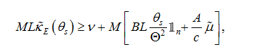
This optimization problem is denoted (O1) and will be solved in two stages. In the first stage we set an objective with and and we search solution of the following optimization problem:
(24a)
subject to:
(24b)
(24c)
(24d)
In the second stage we search among and obtained from the first stage, the couple which minimize the cost function of the optimization problem (24). For this, we solve the following optimization problem:
(25)
which has at least one solution. In cases where multiple solutions exist, we take the solution that corresponds to the smallest .
3.2. Discretization of Optimization Problem (O1)
The way to discretize problem (24) consists in introducing on n points
such that , where . We assume that for any
, there exists a such that . At the operational level, if this condition is not verified, we substitute by the closest . Then we define n
intervals , such that , defined by:
We consider then the space S made of functions that are defined on and constant on each , for . We introduce the approximation operator P defined by:
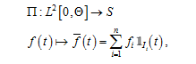 (26)
(26)
where is the mean value of the function f on interval . We denote and we will use these notations afterward for the quan-
tities of the model. We have:
(27a)
(27b)
With this discrete space on hands, we consider the discrete optimization problem that consists in finding solution of (24), with g replaced by , by and by .
It is straightforward to show that, after setting , solving the optimization problem (24) is equivalent to solve the next one.
(28)
where is the set of function satisfying:
(29a)
(29b)
(29c)
with
(30)
and where u is a function that is equal to in each interval , i.e.:
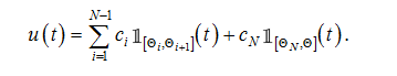 (31)
(31)
Because of the piece-wise constant nature of , we have:
(32)
where matrix , resulting from the convolution, is defined by:
and . Using (32) and (27), operator defined by (15) when applied to yields operator L acting on , defined by:
(33a)
its expression is:
(33b)
with, by using (27):
is the matrix resulting from the approximation of the integral in the formula (15). The constraints given by (29) may then be written as:
 (34a)
(34a)
 (34b)
(34b)
 (34c)
(34c)
where
 ,
, and n is the discretization of (31) given by:
,
, and n is the discretization of (31) given by:
(35)
The discretization of the optimization problem (24) is finally written as the following one.
 (36a)
(36a)
subject to:
 (36b)
(36b)
 (36c)
(36c)
 (36c)
(36c)
Problem (36) is a linear optimization problem which is solved for each , , where , to obtain . Then, among all , we take solution of the following optimization problem:
 (37)
(37)
which has at least one solution. In cases where multiple solutions exist, we take the solution that corresponds to the smallest . We have finally the couple .
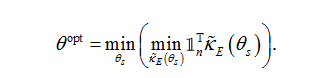
3.2.1. Example 1
In Example 1, as shown in Figure 1, the repayment is done in a constant way between the first and 6th year after borrowing. We pay off nothing outside this period. The current spending density alternates between positive values, corresponding to periods where income is less than spending and negative values, corresponding to periods where income is larger than spending. The optimal loan density and the optimal time to achieve the objective of the project are given in Figure 1. Figure 2 shows that the constraints are satisfied. For this example we have taken:
3.2.2. Example 2
In Example 2, the repayment is only made in an increasing way between the 2nd and 6th year after borrowing. We pay off nothing outside this period. The current spending density alternates between positive values, corresponding to periods where income is less than spending and negative values, corresponding to periods where income is larger than spending. The optimal loan density
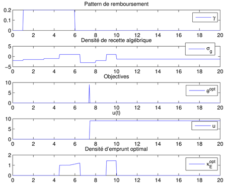
Figure 1. According to the Example 1. Optimal loan and the optimal time obtained for given. repayment pattern g, objectives c and current spending .
Figure 2. Checking if the constraints are satisfied for Example 1.
and the optimal time to achieve the objective of the project are given in Figure 3. Figure 4 shows that the constraints are satisfied. For this example we have taken:
4. Second Optimization Problem (O2)
4.1. Continuous-in-Time Financial Model with Saving
In this model we impose the repayment pattern g, the current spending density , the loan density , the interest rates and . The withdrawal density and the saving density must be chosen such that the current saving field remains non-negative. We then write using (10) the following constraint:
(38)
which can be written:
(39)
However, the isolated spending density must be non negative. Using (16), we have the following inequality:
(40)
From (39) and (40), the two constraints that must be satisfied:

Figure 3. Optimal loan and the optimal time obtained for given. repayment pattern g, objectives c and current spending .
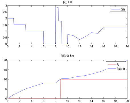
Figure 4. Checking if the constraints are satisfied for Example 2.
(41a)
(41b)
4.1.1. Example 1
In the Figure 5 we show an example of a financial model with saving which the constraints (41) are satisfied. In this example, the repayment is done in a constant way between the first and third year after borrowing. We pay off nothing outside this period. The current spending density alternates between positive values, corresponding to periods where income is less than spending and negative values, corresponding to periods where income is larger than spending. We set the saving density and the withdrawal density as shown Figure 5. For this example we have taken:
4.1.2. Example 2
In the Figure 6 we show an example of a financial model with saving which the constraints (41) are not satisfied. In this example, the repayment is done in a constant way between the first and third year after borrowing. We pay off nothing outside this period. We set the current spending, the saving density and the withdrawal density as shown Figure 6. For this example we have taken:
4.2. Optimization Problem (O2)
The second optimization problem consists to find the optimal variant from the loan density, the saving density and the Withdrawal density obtained from a continuous-in-time financial model with saving. For a given loan density ,
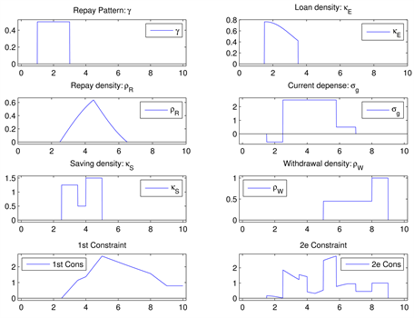
Figure 5. Example of a continuous-in-time financial model with saving (the two constraints (4) are satisfied).
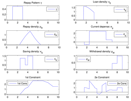
Figure 6. Example of a continuous-in-time financial model with saving (the two constraints (61) is not satisfied).
saving density and withdrawal density which satisfy constraints (41), we want to calculate the positive real numbers a, b and c, such that replacing by , by and by in the initial model, the constraints (41) are still verified. For that we introduce the following optimization problem:
(42)
or
(43)
under the constraints:
(44a)
(44b)
(44c)
To solve this optimization problem with constraints, a quadratic programming method implemented in Matlab is used via the function quadprog. We now apply this optimization problem on the model already presented in Example 0.0.3. We obtain:
The result is shown in Figure 7. This means that among all the financial solutions close to that originally constructed, we take the one that leads to minimize
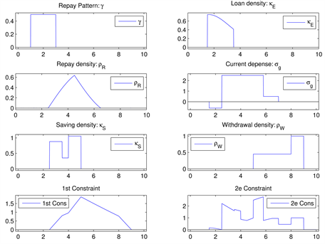
Figure 7. Second optimization problem (O2) applied to the model of Example 1.
the overall amount borrowed, placed and withdrawn. We can also minimize the amount borrowed only by writing the optimization problem in the form:
(45)
We can also minimize the amount borrowed and placed by writing the following optimization problem:
(46)
In the Example 2, the constraint (41b) is not satisfied. However, it is possible, by modifying , and to get another model satisfying constraints (41), by applying the same optimization method. We obtain:
The result is shown in Figure 8.
5. Conclusion
In this paper we have presented an optimal control for a continuous-in-time financial model which is designed to be used for the finances of public institutions. This model describes the loan, reimbursement, saving and interest payment schemes; and uses mathematical operators to describe links existing between those quantities. The aim of the optimal loan strategy is to minimize the interest payment taking into account the objective of the project, the incomes, the saving and the spending. We have built a mathematical framework for the optimal control problem which consists to solving a constraint optimization problem. Two optimization problems were introduced in this paper. The first
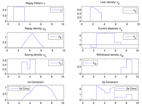
Figure 8. Second optimization problem (O2) applied to the model of Example 2.
one which is introduced in Section 3 consists in finding a loan scheme minimizing the cost of the loan for a project, together with the time to achieve its objectives. The second optimization problem which is introduced in Section 4 consists, from given loan, saving and withdrawal schemes, to finding optimal variants of them. In order to solve these optimization problems we have used simplex and quadratic methods. The numerical simulations were performed by using the mathematical software of scientific computing Matlab. The simulations’ results are consistent with the theoretical part and show the performance and stability of our approach.
Acknowledgements
This work is jointly funded by MGDIS company (http://www.mgdis.fr/) and the PEPS program Labex AMIES (http://www.agence-maths-entreprises.fr/).
Cite this paper
Frénod, E., Ménard, P. and Safa, M. (2018) Paper Title. Journal of Mathematical Finance, 8, 27-42. https://doi.org/10.4236/jmf.2018.81003
References
- 1. Frénod, E., Ménard, P. and Safa, M. (2017) Optimal Control of a Continuous-in-Time Financial Model. American Journal of Modeling and Optimization, 5, 1-11.
- 2. Frénod, E. and Safa, M. (2014) Continuous-in-Time Financial Model for Public Communities. ESAIM: Proceedings and Surveys, 45, 158-167. https://doi.org/10.1051/proc/201445016
- 3. Frénod, E. and Chakkour, T. (2016) A Continuous-in-Time Financial Model. Mathematical Finance Letters, 37, 2051-2929.
- 4. Merton, R.C. (1992) Continuous-Time Finance. Blackwell, Cambridge, MA.
- 5. Sundaresan, S.M (2000) Continuous-Time Methods in Finance: A Review and an Assessment. Journal of Finance, 55, 1569-1622. https://doi.org/10.1111/0022-1082.00261
- 6. Keel, S.T. (2006) Optimal Portfolio Construction and Active Portfolio Management Including Alternative Investments. PhD Thesis, Swiss Federal Institute of Technology Zurich, Zurich.
- 7. Grigorieva, E.V. and Khailov, E.N. (2005) Optimal Control of a Commercial Loan Repayment Plan. Discret and Continuous Dynamical Systems, 2005, 345-354.