Received 17 January 2014; revised 26 February 2014; accepted 11 March 2014

ABSTRACT

To capture the impact of skewness and increase kurtosis on Black’s [1] European put values, we first substitute a Gram-Charlier (GC) distribution and next a Johnson distribution for Black’s Gaus- sian one. We introduce next each distribution in the option payoff and develop until the closed- form expression of each put is arrived at. Finally, we estimate by simulations GC, Johnson and Black put options, choosing the latter one as benchmark. Simulation estimates encompassing both skewness and kurtosis show that, for at-the-money (ATM) or slightly in-the-money put values, 1) Black’s overvaluation with respect to Johnson puts is very significant and 2) its undervaluation with respect to GC ones remains moderate. Yet, by using the same skewness values for both GC and Johnson puts, we highlight the differences induced by increasing kurtosis between the two models. In this case, the GC overvaluation for ATM values is explained by value differences in the put time component. Yet, while both Black and GC values exhibit significant time decay close to expiry, Johnson’s ones remain stable up to maturity.

Keywords:

Skewness and Increasing Kurtosis in Gram-Charlier (GC) and Johnson Distributions, At-the-Money overvaluation of Black’s but Undervaluation of GC European Futures Put Values in terms of Johnson’s Ones, Value differences Explained by the Put time Component

1. Introduction

This paper offers a solution to the following problem: how to account for skewness and extremely large Pearso- nian kurtosis (up to 39) when estimating a European put option embedded in a non-traded asset (a bank’s credit- line commitment) subject to Basel III capital sufficiency? There are two steps to the solution: first to determine the four-parameter analytical solution of the put option and then to use it to value the credit risk of banks’ loan commitments.

In option finance, numerous empirical studies have shown that the log-return distribution exhibits positive or negative skewness coupled with various degrees of positive excess kurtosis. It thus makes sense to consider moving away from the Gaussian distribution underlying Black’s [1] European futures put option―the choice of this option type is dictated by the case study examined later on. The procedure oftentimes used to account si- multaneously for skewness and kurtosis is a Gram-Charlier (GC) type-A statistical-series expansion of the un- derlying asset log-return risk-neutral density function, truncated after the fourth moment. While widely used and often relevant, the expansion presents at least three significant limitations. Firstly, the values of the skewness and kurtosis parameters are restricted to an admissible elliptical region defined by Barton and Dennis [2] and re- visited more recently by Schlögl [3] ¹. Secondly, the truncated expansion may not converge to the true value and may only approximate the unknown distribution. Thirdly, adding more terms in an orthogonal expansion may not necessarily mean greater accuracy: it is known that higher-order approximations may become more and more oscillatory.

So, as first improvement, let us consider replacing the GC expansion by a “true” GC distribution, namely a generalized GC distribution of which the density function is of the same form as the expansion―a normal den- sity times a polynomial. The latter true probability density function (pdf) has the advantage to be nonnegative, integrate to one and be of an even order―if it were odd the polynomial would take negative values for some x. Among the generalized GC distributions, we then focus on the GC four-moment family: The latter is then intro- duced in the option payoff which is developed until the closed-form expression of the European put option is ar- rived at. This expression will be referred to as the GC put option. The procedure is attractive as long as the lep- tokurtic distribution presents moderate kurtosis, namely no larger than 7. Yet, many of the distributions of well-known indices underlying options do exhibit positive or negative skewness combined with more severe kurtosis, in the range of 10 to 25. To wit, kurtosis values up to 10 are reported by Jha and Kalimipalli [5] for the distribution of S&P500 returns over the period 1990 to 2002. Kurtosis values of 10 are also reported by Polanski and Stoja [6] for the Dow-Jones daily returns over the period September 2000 to August 2008. In [7] , Chalaman- drias and Rompolis are extracting the implied kurtosis values from European options on the S&P500 index for the years 1996 to 2007: some of the values are as high as 17.4. Recently finally, Del Brio and Perote [8] reported a kurtosis value as high as 25.0063 for the Dow-Jones returns over the very long period of October 1928 to April 2009. The case study examined here differs from these studies to the extent that it deals with an embedded put option on an underlying non-traded bank instrument of which the log-return distribution exhibits kurtosis values as large as 39.

In view of this empirical evidence, our quest then narrows down to finding another distribution that accom- modates more severe excess kurtosis. This distribution is based on Johnson’s translation method [9] ² by which the transformed variate becomes at least approximately normal. Matching frequency curves is used as follows. Select the appropriate translation system so that the first four moments of the true distribution of variable x match those of an approximated distribution, say z. Compute next the four parameters of the latter distribution, introduce it in the option payoff and develop so as to arrive at a closed-form expression of the European put op- tion. This analytical expression will be referred to as Johnson’s put option. The latter analytics show that excess kurtosis mainly affects the time component of the put value.

To assess the benefits of GC and Johnson put options, the real-world case of the European put option embed- ded in banks’ credit line commitments is examined. It is first explained how the commitment value (to be re- ferred to as the indebtedness futures value) gives rise to the implicit European futures put option. The latter put is next valued by simulation under the Gaussian distribution, the true GC distribution and Johnson’s mo- ment-matching distribution, respectively. These put values are computed as a function of both indebtedness val- ue and option term, with Black’s put chosen as benchmark. Regarding the combined effect of skewness and kurtosis, the simulations reveal that, for at-the-money (ATM) or slightly in-the-money (ITM) indebtedness values, Black’s put values are greater than Johnson’s ones but smaller than GC’s ones. In the sequel, we speak of over- or undervaluation for the sake of simplicity and clarity. For deeper ITM indebtedness values, however, Black’s over- valuations with respect to both Johnson and GC estimates is minimal, though slightly more pronounced in GC’s case. The sole effect of increasing kurtosis is captured by the differences between GC and Johnson put values when the values of skewness and the other parameters are kept the same for both options. Here again, the GC over- valuation is greatest for ATM or slightly ITM values and an insightful explanation is provided. It is also worth- while examining how the put value is decaying over the option last two months for ATM or slightly ITM values. Does the rapid time decay of Black’s put value also extend to the GC and Johnson’s values?

The layout of the paper is as follows. Section 2 is devoted to the derivation of the European put options based on GC or Johnson four-parameter distributions. Section 3 examines the real-world situation of the European fu- tures put option embedded in a credit-line commitment. In the first subsection, the credit-line indebtedness value is derived and the statistical evidence regarding its log-returns is presented. The second one explains the choice of simulation parameters as well as the meaning of the put estimates. The third one assesses value differences between GC, Johnson and Black put options arising from skewness and excess kurtosis. Short concluding re- marks close the paper in Section 4.

2. Valuing the European Put Option under Skewness and Increasing Excess Kurtosis

We choose Black’s [1] European futures put option, P_B (a choice conditioned by the case-study illustration) as starting point as well as benchmark for future comparisons. Namely:

(1)

with

where F₀ denotes the date-0 underlying futures value; K, the exercise value; d₁, the standard moneyness with N(.), the cumulative distribution function of the standard normal distribution; r, the short-term risk-free rate of interest³; s, the standard deviation of the futures value; and T, the put expiration date. The log-return distribution underlying Black’s put option being Gaussian, skewness is nil and Pearsonian kurtosis is equal to three.

Our quest thus is: How can we improve on Black’s put option by varying skewness and kurtosis away from their Gaussian values? While a rich literature exits regarding option models with stochastic volatility, stochastic interest rate, with or without jumps (see Bakshi, Cao and Chen [16] or Heston and Nandi [17] among the nu- merous references), the most prevalent way of valuing options encompassing four moments is the Gram-Char- lier approach: see among others, Schlögl [3] , Del Brio and Perote [8] , Chateau [15] , Backus, Foresi, Li and Wu [18] , Bakshi and Madan [19] , Corrado [20] , Corrado and Su [21] , Jurczenko, Maillet and Negrea [22] , and Ta- naka, Yamada and Watanabe [23] . The procedure relies on an A-type Gram-Charlier truncated statistical-series expansion of the underlying price change relatives; yet the expansion only becomes an actual density if the Jon- deau-Rockinger [4] joint constraint on skewness and kurtosis coefficients is satisfied. Numerically, the skewness and kurtosis coefficients ought to lie in the intervals [−1.0493, 1.0493] and [3] , [7] respectively, so as to prevent negative probabilities in the tail of the distribution. Beyond this limitation, there are at least another two other good reasons for substituting a “true” distribution to the GC expansion. Firstly, the truncated GC series expan- sion may not converge to the true value and may only approximate the unknown distribution. Secondly, adding more terms in an orthogonal expansion may not necessarily mean greater accuracy: it is known that higher-order approximations may become more and more oscillatory. Technically, we propose to go from a [truncated] ex- pansion to a generalized GC distribution, with both having a density function of the form of a normal distribu- tion times a polynomial: namely

where

and

with He_k referring to the Hermite polynomial of order k. We then introduce the GC distribution in the option payoff and derive the analytical form of the four-parameter GC European futures put value that satisfies the martingale constraint (see for instance Corrado [20] or Harrison and Pliska [24] ), as is done in Appendix A. The resultant closed-form solution is labeled the GC put value:

(2)

where

(3)

with

and

where μ₃ and μ₄ denote the centered moments of order i, for i = [3, 4], and ω accounts for these moments in the put standard moneyness. In addition

(4)

and

(5)

More concretely, the GC put value P_GC in Equation (2) is a Black European put option, P_B, minus terms for non-normal skewness and kurtosis. Here the GC distribution does influence directly the skewness and kurtosis coefficients.

In practice, while skewness values oftentimes are falling within the constrained interval, kurtosis values range way beyond seven, the upper-bound value of the constrained GC distribution. A first improvement can be found in a subset of the order-2m GC family introduced by Leon, Mencia and Santana [25] . For semi-nonparametric distributions, the authors’ Figure 1 presents skewness-cum-kurtosis envelopes which are wider than the Jondeau- Rockinger admissible region. While their various regions can accommodate kurtosis values up to 15 for op- tion-relevant skewness values, the figure clearly shows that the frontier is open-ended for higher kurtosis values ―more specifically values between 24 and 39 to be encountered in the subsequent case study. Such values are not unheard of as mentioned in the introduction. Yet even more extreme kurtosis values were recently reported by Cayton and Mapa (Table 4, Page 20) in [10] : coefficients of 115.22 and 43.30 of the distributions of the re- turn time series of the Philippines Peso-US$ and Philippines Peso-Euro exchange rates over the period January 1999 to November 2011.

Our quest thus then narrows down to: Does a distribution other than the generalized GC distribution exist that accounts for kurtosis values larger than 7 let alone 20? The solution is to be found in a particular family of fre- quency curves generated by Johnson’s translation system [9] . The steps are as follows. Use the relevant transla- tion system so that the first four moments of the distribution of variable x match those of any required distribu- tion, say here z. Compute next the four parameters of the approximated distribution, introduce the latter one in the option payoff and develop until the analytical expression of the European futures put option is arrived at. These travails are presented in Appendix B: the resultant closed form is labeled Johnson’s European futures put value, P_J:

(6)

where γ, δ, ξ, and λ are the four parameters of the unbounded translation system S_U defined in Appendix B,

with sinh^‒1 the inverse of the hyperbolic sine function, the other terms having

been defined previously. In contrast with the GC distribution, Johnson’s S_U distribution does not influence di- rectly the coefficients of skewness and kurtosis. Yet, Johnson’s put is appealing since it accounts for all kurtosis values versus a maximum of 7 for the constrained Gram-Charlier distribution. There is no pretense on our part that moment fitting be regarded as providing the “best” solution in any sense. The more modest claim is that fitting by moments improves on the distribution-based GC approach and produces some significant put-value differences as evidenced from the credit-commitment case study of the next section.

3. Case Study: Of the Credit-Risk Put Option Embedded in Banks’ Credit Line Commitments

3.1. The European Put Option Embedded in short-term Commitments and the Statistical evidence regarding Indebtedness-value Change relatives

Since Thakor, Hong and Greenbaum [26] , the credit risk of loan commitments is apprehended by an embedded put option that is used to compute the risk-weighted amount of commitments subject to Basel III capital re- quirements (see Basel Committee on Banking Supervision [27] ). For understanding the case study, three fea- tures of this embedded European futures put option are reviewed: the origin of the implicit put option, why it is European, and how the put term to maturity also endogenizes credit line draw-down⁴.

A bank credit-line commitment allows a borrower to draw, say, over a one-year period [0, T] up to K = $100 at a floating prime rate defined as namely a date-0 fixed markup plus a date-T (when funding takes place) stochastic cost of funds. It is the fixed markup of the floating prime rate that generates the embedded put option, for any prime-rate borrower can secure date-0 funding either through a credit-line commitment or a demand loan characterized by a stochastic spot markup (denoting the spot floating prime rate and the bank’s funding rate in the banker’s acceptances market). Fixed and variable markups enable us to define the j-month-old indebtedness futures⁵ value F_j as:

, (7)

where is the difference between the date-0 fixed markup and the date-j variable markup, is loan duration (one year) once the commitment has been exercised and K is the constant line par value. For in- stance, for an initially one-year commitment (to fix ideas, say, from July 1st to June 30^th), F₆ denotes a six- month-old indebtedness value which still has a remaining six-month term to maturity. The F_js are the values of the banking instrument underlying the put in Equations (1), (2), and (6), of which the date-T payoff is

Suppose next that:

1) At year end, namely the date at which the bank’s audit under Basel III regulation takes place (see Basel Committee on Banking Supervision [27] ), j-month old commitments have various remaining time to expiry. By making date j the option valuation date and by assuming for clarity that it coincides with Basel yearend audit date, then the time remaining to commitment expiry becomes the remaining life of contract―as Merton has ar- gued for related loan guarantees in [33] . For instance, our one-year (July to June) commitment is 6-month old at the end of December when the Basel audit takes place, so generating a 6-month put option. Thus, it is the Basel framework that makes the put option European⁶.

2) At valuation date j, suppose that the fluctuations in the spot markup of the floating prime rate on demand loans result in. According to Equation (7), the rational commitment holder then decides to draw on the line because its fixed markup is less than the stochastic spot markup. To wit, if a 2.0% fixed markup is combined with, say, a 3.0% spot markup, Equation (7) gives rise to an implicit put option as the borrower’s debt value F_j is less than the option strike price K. When, the rational borrower chooses a spot loan instead of drawing on the credit line commitment; in that case, there is no embedded put and hence no impact regarding Basel risk-weighted assets. In short, spot markup fluctuations at valuation date j give rise to a j-month European put option embedded in an initially one-year line commitment. Moreover, the put term to maturity enable us to endogenize the credit line take-down: at date j, the borrower can still draw on the line unused portion for the forward period T ‒ j. And the longer this forward period, the greater the borrower’s potential line draw-down. The latter thus becomes a function of the line remaining term. In short, the commitment put being both a func- tion of indebtedness value and term, put estimates will be reported as a matrix or shown as a put-value surface.

Given Equation (7), let us now consider the distribution of the monthly log returns of the indebtedness value. Namely

(8)

where _tF(j) is the date-t value of the j-month-old indebtedness value. Expression (8) thus generates a time series of monthly change relatives from an indebtedness value that remains continuously j-month-old. The log-F rela- tives from the third to the ninth month are listed in Exhibit 1. From the statistical evidence presented in the third column, the volatility of the empirical distributions fluctuates in the narrow range [1.51% p.a. to 1.63% p.a.] for log-F relatives computed for the selected months. The confidence intervals for the normal sample skewness and kurtosis coefficients with 300 observations are computed in the note at the bottom of the exhibit. According to the statistics shown in the fourth and fifth columns, several positive and negative skewness coefficients as well as all kurtosis values fall outside their respective confidence intervals. This indicates that the empirical distribu- tions present mostly weak asymmetry coupled with an extremely strong leptokurtic pattern (very severe Pearso- nian kurtosis). Since the indebtedness value is a non-traded banking instrument, the historical values of the vola- tility, asymmetry and kurtosis coefficients from Exhibit 1 will be used in the next subsection, in which the put option reflecting commitment credit or spread risk is priced.

3.2. Simulation parameters and Estimate Meaning

The embedded put values are estimated by simulations based on the statistical evidence presented in Exhibit 1. From the information reported in its columns 6 and 7, nearly all indebtedness values vary between $96.2 and $104.1, with $100 being par value; we thus set F_j at $100, $99.5, $99, $98.5, $98, and $97.5⁷ for a commitment put that moves progressively in the money. For these indebtedness values, the simulations are performed for commitments with strike price K = $100, short-term risk-free rate r = 3% p.a., remaining terms to maturity (T ? j) from 3 to 9 months, and volatility and skewness values from Exhibit 1. Regarding Gram-Charlier puts, we choose a kurtosis value of 6.5 which, while just remaining under the Jondeau-Rockinger upper bound, still accommodates the skewness estimates of Exhibit 1. As for Johnson’s put values, we use Tuenter’s [34] iterative procedure which allows for the much greater kurtosis values reported in Exhibit 1.

Before commenting on the simulation patterns, we clarify the meaning of our slightly in-the-money reference scenario, namely the European put value of which the entries are F = $99 and T ? j = 6 months in the first matrix of Table 1. This cell corresponds to a credit-risk put of which the indebtedness value F = $99 is slightly ITM with six months remaining to commitment expiry. According to the (underlined) estimate P_J = $0.985, the Johnson put has an equilibrium value of slightly less than 1% per $100 of commitment if the floating prime-rate commitment with say a 2.0% p.a. fixed markup is priced when the same-date spot-loan stochastic markup is 3.0% p.a. On the other hand, Black and Gram-Charlier corresponding put values, P_B = $1.101 and P_GC = $1.092 in the table second and third matrices respectively, are larger and thus most likely overvalued in terms of P_J. Table 1 matrices can be mapped into put-value surfaces, of which the base axes are risk (corresponding to the in- debtedness value down the matrix columns) and term (the remaining time to put maturity shown across the matrix rows), respectively⁸. For illustrative purpose, the first (Johnson) matrix is shown in Chart 1. Its visual

Exhibit 1. Statistical analysis of the 300 monthly observations of the time series of indebtedness-value change relatives computed with Equation (8) for the period from 1988.01 to 2012.12.

^AMonthly unbiased (divided by n-1) value × √12 = sigma in percent per annum. Note: For a sample size n = 300 observations, the 95% confidence intervals for normal sample coefficients of skewness and kurtosis are: ±1.96 (6/300)^1/2 = ±0.277 and 3 ± 1.96 (24/300)^1/2 = 3 ± 0.554, respectively. Source: Statistics Canada monthly time series V122495 and V122504 of the prime credit rate and one-month banker’s acceptance rate of chartered (commercial) banks, respectively.

Note: Matrix P_J: Johnson’s European futures put values from Equation (6). Matrix P_B: Black’s European futures put values from Equation (1). Matrix P_GC: Gram-Charlier’s futures put values from Equation (2). Parameter definition: F = indebtedness futures value in $ computed from Equation (7); K = $100 the credit-line exercise value; r = short-term risk-free rate of interest, in % per annum; T = commitment maturity date; and T ‒ j = time remaining to commitment put expiry, in months. Common parameters: L = 100; r = 0.03; T ? j = 3,…, 9 months with T = 12 months. The volatility, skewness and kurtosis parameter values are from columns 3 to 5 of Exhibit 1.

inspection reveals that the straight put-value surface is down-sloping implying that Johnson’s put values are far more driven by risk changes than by maturity changes (namely not significantly tilted in the term-to-maturity dimension). Similar but slightly curved down-sloping surfaces (not shown here) depict the GC and Black put- value matrices.

3.3. Assessing Values differences between Black, GC and Johnson Puts arising from Skewness and excess kurtosis

Value differences due to the joint impact of skewness and kurtosis on put values are examined first. Selecting Black’s put value as benchmark, the differences [P_B ? P_J]/P_B and [P_B ? P_GC]/P_B, namely Black’s percentage dif- ferences with respect to Johnson’s and GC put values, highlight the departures from the Gaussian distribution. These are shown in the first and second matrices of Table 2. The latter visual inspection reveals that, for ATM

Chart 1. Surface of Johnson’s at- and in-the-money European futures put values as a function of risk and term.

Note: Matrix (P_B ‒ P_J)/P_B: Johnson’s differentials with respect to Black’s put values. Matrix (P_B ‒ P_GC)/P_B: Gram-Charlier’s differentials with respect to Black’s put values. Matrix (P_GC ‒ P_J)/P_GC: Johnson’s differentials with respect to Gram-Charlier’s futures put values. Parameter definition: P_B: Black’s European futures put values from Equation (1); P_GC: Gram-Charlier’s futures put values from Equation (2); P_J: Johnson’s European futures put values from Equation (6); F = indebtedness futures value in $ computed from Equation (7); and Term = time remaining to commitment put expiry, in months.

or slightly ITM indebtedness values, Black’s put values overestimate Johnson’s ones but underestimate GC’s ones. Percentage wise, Black’s overvaluation with respect to Johnson values is much greater (ranging up to 99.07%) than the undervaluation with respect to GC values (ranging up to 27.29%). For deeper ITM indebted- ness values, Black’s overvaluations with respect to both Johnson and GC are minimal, with those with respect to GC’s values slightly larger than those with respect to Johnson’s values. By way of contrast, the table third matrix highlights the kurtosis-induced differences between GC and Johnson put values (skewness and the other parameter values being then kept identical for both puts), namely [P_GC ? P_J]/P_GC. This matrix is also mapped into Chart 2 below. Recall that for GC put values, kurtosis was fixed at 6.5 while it ranges from 24.16 to 39.34 for Johnson’s ones in Exhibit 1. In Chart 2, the GC largest overvaluation (99.23%, close to the front upper left corner of the chart) takes place when the indebtedness value is ATM with 8-month re- maining to maturity. Yet, overvaluation turns into slight undervaluation for deeper ITM indebtedness values, witness the 2.71% undervaluation for the longest remaining term (9 months)―in the front lower corner of the chart.

Now why are the differences between Johnson and Black and Gram-Charlier put values largest for ATM in- debtedness values? According to the developments in Appendix B, it is the time value of the Johnson put that makes all the difference. As for any option, this time value usually happens to be largest for the ATM value. But as the ATM time value is smallest for the Johnson put relative to the Black and Gram-Charlier ones, this is where their value differences are greatest. But for deeper ITM put values, the time-induced value differences between the three procedures dwindle significantly. Moreover, changes in the ATM put values over the last two months before expiry provide some additional insight. For Black’s put, it is well-known that the ATM values are rapidly decaying over the option last two months. Exhibit 2 presents for the reference scenario (the put with six months left to maturity in Table 1) the values of Black, GC and Johnson puts two months, one month and two weeks before expiry.

While both Black’s and GC’s ATM values decay rapidly over the two last months, Johnson values remain remarkably stable throughout at the much lower level of about half a cent. For the slightly in-the-money values, Johnson’s ATM put values also remain stable about 50 and 99 cents respectively. Yet, while Black’s and GC’s

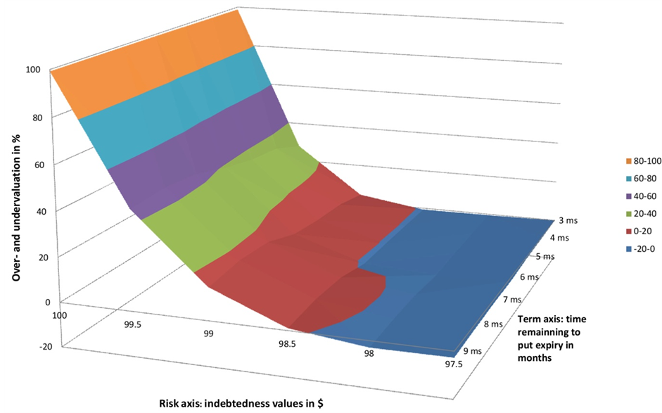
Chart 2. Over- and undervaluation of Gram-Charlier’s European futures put values with respect to Johnson’s corresponding ones: Values differences as a function of risk and term.

Exhibit 2. Black, GC and Johnson at- or slightly in-the-money put values, expressed in dollars.

values remain larger than Johnson’s ones, they are slowly converging to Johnson’s ones, with two weeks re- maining to maturity. Practically, other things remaining constant, long-position holders of Black’s and GC puts should sell their positions preferably two months before maturity so as to avoid losing time value. On the other hand, holders of long Johnson’s puts can maintain theirs without any loss of time value.

So, we suggest the following heuristic explanation for such ATM time differences. With a very leptokurtic distribution, Johnson put values are bunched close to the peak of a density function that does not exhibit much volatility, and may or may not have thick tails. Thus using a distribution that allows for increasing kurtosis val- ues reduces the time value of ATM or slightly ITM European futures put options; this is the case of Johnson’s approach as it is able to accommodate higher levels of kurtosis. In other words, Johnson distributions may be well-suited to time series in which value changes over time take place in a narrow band as for interest rates or are range-bound as in the case of many default-free bonds. Needless to say, additional empirical studies cover- ing traded options with different underlying financial instruments should be considered so as to corroborate the patterns evidenced for an embedded put option on a non-traded underlying bank instrument.

4. Concluding Remarks

To capture the impact of skewness and increasing kurtosis on values of Black’s [1] European put options, the paper proposes to first substitute a “true” Gram-Charlier (GC) distribution and next a moment-matching Johnson distribution for Black’s Gaussian one. In the first case, the generalized GC distribution substitutes for the often- used GC truncated expansion as the latter may not converge to the true value and may only approximate the un- known distribution. However, the GC four-parameter density function selected limits excess kurtosis to the val- ue of four. To account for more severe excess kurtosis, another distribution based on Johnson’s moment- matching approach is introduced: the four parameters of the translated distribution are then introduced in the op- tion payoff which is developed until the closed-form of the European futures put option is arrived at.

Next Black, GC and Johnson estimates of the European put option embedded in credit line commitments are obtained by simulations, with Black’s put option selected as benchmark. Regarding the combined effect of skewness and kurtosis, the simulations reveal that, for at-the-money (ATM) or slightly in-the-money (ITM) in- debtedness values, Black’s European put values overestimate Johnson’s ones but underestimate GC’s ones. For deeper in-the-money indebtedness values, however, Black’s overvaluations with respect to both Johnson and GC are minimal, although slightly more pronounced in GC’s case. The sole effect of increasing kurtosis is captured by the differences between GC and Johnson put values when the values of skewness and the other parameters are kept the same for both options. Here again, the GC overvaluation is most significant for at- or slightly in-the-money indebtedness values because the time component of Johnson’s put is smaller than that of Black’s or GC’s. Thus using a distribution that allows for increasing kurtosis values reduces the time value of ATM or slightly ITM European futures put estimates; this is more evident for Johnson’s approach since it is able to ac- commodate higher levels of kurtosis. This pattern seems characteristic of very peaked distribution with low vo- latility. Such distributions can be found for default-free bonds or interest-rate time series in normal circums- tances. Additional empirical studies covering traded options with different underlying financial instruments should be considered so as to corroborate the patterns evidenced in this case study. This constitutes one of the avenues for further study.

Acknowledgements

For helpful comments and discussions, I thank Daniel Dufresne, Anatole Joffe, Steven Lo, Lewis Tam, and par- ticipants to a research seminar at the University of Macau, China, the 2013 Conference in Mathematical Finance in Montreal, Canada, and the 2013 Conference on Quantitative Methods in Finance in Sydney, Australia.

References

NOTES

¹Barton and Dennis [2] and Jondeau and Rockinger [4] deal with the constrained four-moment GC expansion. For a GS expansion involving k moments with k even and larger than four, Schlögl [3] proposes a calibration algorithm that also yields a valid probability density.

²Among previous applications in finance of Johnson’s translation system, consult Cayton and Mapa [10] , Guldiman [11] , Longerstaey and Spencer [12] and Simonato [13] for value-at-risk, and Posner and Milesky [14] for exotic options.

³In an additive floating-rate commitment (cost of funds + spread), the commitment put only apprehends spread or credit risk; the cost of funds or interest-rate risk is borne by the borrower, not the bank. Any bank market risk is dealt with separately as operational risk in Basel III, as in Chateau [15]. Moreover, cost of funds and spread being weakly and negatively correlated, it is appropriate using r as discount factor in the put equation.

⁴This cursory description only focuses on the analysis-relevant features of credit-line commitments. For more detailed developments, consult articles devoted to credit line commitments such as Thakor, Hong and Greenbaum [26] , Chava and Jarrow [28] , Saunders and Cornett [29] , Standhouse, Schwarzkopf and Ingram [30] or Thakor [31] .

⁵We speak of a futures value for at least three good reasons. Since the bank contracts up to $100 at date t = 0 and delivers up to $100 at T, it is better to speak of indebtedness forward/futures value than of indebtedness spot value as in Thakor, Hong and Greenbaum [26] . The spread is an additive quasi-market value since it is the difference between the prime rate and the rate on bankers’ acceptances, both being market variables. Finally, for short contracts of a few months, there always exists a zero-coupon bond or a Treasury note corresponding to the monthly maturity; differences between forward and futures prices then are sufficiently small to be ignored (see Hull [32] ).

⁶There also exits an American commitment put option of interest to the bank’s day-to-day management. But for computing Basel capital charge corresponding to commitment markup (credit) risk, the relevant put is the European one.

⁷In-the-money indebtedness values below $97.5 are of limited interest since, according to the last column of Exhibit 1, there are never more than a few values (outliers) lower than $97.5 out of the 300 monthly observations.

⁸Heuristically, the put value constitutes the cost incurred by the bank for carrying from Basel fixed audit date onwards unused lines with va- rying remaining term to maturity. The varying term captures the fact that borrowers can draw larger amounts if the credit line remaining time to expiry is longer.

⁹As is usually done in incomplete markets, we specify the underlying distribution under Q from the start, leaving P unspecified (see Harrison and Kreps [36], the finite case, Page 393). Pricing is done under a specific G-C distribution describing “the” risk-neutral measure. The log- returns distribution does not have to be of the same type under both measures; all that is needed is that the support of the log-returns distribu- tion under P be the whole real line, as it is under Q.

References

- 1. Black, F. (1976) The Pricing of Commodity Contracts. Journal of Financial Economics, 3, 167-179.
http://dx.doi.org/10.1016/0304-405X(76)90024-6 - 2. Barton, D.E. and Dennis, K.E.R. (1952) The Conditions under Which Gram-Charlier and Edgeworth Curves are Positive Definite and Unimodal. Biometrika, 39, 425-427.
- 3. Schlogl, E. (2013) Option Pricing Where the Underlying Assets Follow a Gram-Charlier Density of Arbitrary Order. Journal of Economic Dynamics and Control, 37, 611-632.
http://dx.doi.org/10.1016/j.jedc.2012.10.001 - 4. Jondeau, E. and Rockinger, R. (2001) Gram-Charlier Densities. Journal of Economic Dynamics and Control, 25, 1457-1483.
http://dx.doi.org/10.1016/S0165-1889(99)00082-2 - 5. Jha, R. and Kalimipalli, M. (2010) The Economic Significance of the Conditional Skewness in Index Option Markets. Journal of Futures Markets, 30, 378-406.
- 6. Polanski, A. and Stoja, E. (2010) Incorporating Higher Moments into Value-at-Risk Forecasting. Journal of Forecasting, 29, 523-535.
http://dx.doi.org/10.1002/for.1155 - 7. Chalamandrias, G. and Rompolis, L.S. (2012) Exploring the Role of the Realized Return Distribution in the Formation of the Implied Volatility Smile. Journal of Banking and Finance, 36, 1028-1044.
http://dx.doi.org/10.1016/j.jbankfin.2011.10.016 - 8. Del Brio, E.B. and Perote, J. (2012) Gram-Charlier Densities: Maximum Likelihood versus the Method of Moments. Insurance: Mathematics and Economics, 51, 531-537.
http://dx.doi.org/10.1016/j.insmatheco.2012.07.005 - 9. Johnson, N.L. (1949) Systems of Frequency Curves Generated by Methods of Translation. Biometrika, 36, 149-176.
- 10. Cayton, P.J. and Mapa, D.S. (2012) Time-Varying Conditional Johnson SU Density in Value-at-Risk (VaR) Methodology. MPRA Paper No 36206, University of the Philippines at Diliman, Philippines.
- 11. Guldiman, T. (1997) Risk Metrics Technical Document. Morgan Guarantee Trust Company, New York.
- 12. Longerstaey, J. and Spencer, M. (1996) Risk MetricsTM. Technical Document, J.P. Morgan/Reuters, New York.
- 13. Simonato, J.-G. (2011) The Performance of Johnson Distributions for Computing Value at Risk. Journal of Derivatives, 19, 7-24.
http://dx.doi.org/10.3905/jod.2011.19.1.007 - 14. Posner, S.E. and Milesky, M.A. (1998) Valuing Exotic Options by Approximating the SPD with Higher Moments. Journal of Financial Engineering, 7, 109-125.
- 15. Chateau, J.-P. (2009) Marking-to-Model Credit and Operational Risks of Loan Commitments: A Basel-2 Advanced Internal-Ratings Based Approach. International Review of Financial Analysis, 18, 260-270.
http://dx.doi.org/10.1016/j.irfa.2009.07.001 - 16. Bakshi, G., Cao, C. and Chen, Z. (1997) Empirical Performance of Alternative Option Pricing Models. Journal of Finance, 52, 2003-2049.
http://dx.doi.org/10.1111/j.1540-6261.1997.tb02749.x - 17. Heston, S.L. and Nandi, S. (2000) A Close-Form GARCH Option Valuation Model. Review of Financial Studies, 13, 585-625.
http://dx.doi.org/10.1093/rfs/13.3.585 - 18. Backus, D., Foresi, S., Li, K. and Wu, L. (2004) Accounting for Biases in Black-Scholes. Working Paper, New York University, New York.
- 19. Bakshi, G. and Madan, D. (2000) Spanning and Derivative-Security Valuation. Journal of Financial Economics, 55, 205-238.
http://dx.doi.org/10.1016/S0304-405X(99)00050-1 - 20. Corrado, C.J. (2007) The Hidden Martingale Restriction in Gram-Charlier Option Prices. Journal of Futures Markets, 27, 517-534.
http://dx.doi.org/10.1002/fut.20255 - 21. Corrado, C.J. and Su, T. (1996) Skewness and Kurtosis in S&P 500 Index Returns Implied by Option Prices. Journal of Financial Research, 19, 175-192.
- 22. Jurczenko, E., Maillet, B. and Negrea, B. (2004) A Note on Skewness and Kurtosis Adjusted Option Pricing Models Under the Martingale Measure. Quantitative Finance, 4, 479-488.
- 23. Tanaka, K., Yamada, T. and Watanabe, T. (2010) Applications of Gram-Charlier Expansions and Bond Moments for Pricing of Interest Rates and Credit Risk. Quantitative Finance, 10, 645-662.
http://dx.doi.org/10.1080/14697680903193371 - 24. Harrison, J.M. and Pliska, S. (1981) Martingales and Stochastic Integrals in Theory of Continuous Trading. Stochastic Processes and Their Applications, 11, 215-260.
http://dx.doi.org/10.1016/0304-4149(81)90026-0 - 25. Leon, A., Mencia, J. and Sentana, E. (2009) Parametric Properties of the Semi-Nonparametric Distributions, with Applications to Option Valuation. Journal of Business and Economic Statistics, 27, 176-192.
http://dx.doi.org/10.1198/jbes.2009.0013 - 26. Thakor, A.V., Hong, H. and Greenbaum, S.I. (1981) Bank Loan Commitments and Interest Rate Volatility. Journal of Banking and Finance, 5, 497-510.
http://dx.doi.org/10.1016/S0378-4266(81)80004-0 - 27. Basel Committee on Banking Supervision (2013) Progress Report on Basel III Implementation. Bank for International Settlements, Basel, April 2013.
- 28. Chava, S. and Jarrow, R. (2007) Modeling Loan Commitments. Finance Research Letters, 5, 11-20.
http://dx.doi.org/10.1016/j.frl.2007.11.002 - 29. Saunders, A. and Cornett, M.M. (2011) Financial Institutions Management: A Risk Management Approach. 7th Edition, Irwin/McGraw-Hill, New York.
- 30. Standhouse, B., Schwarzkopf, A. and Ingram, M. (2011) A Computational Approach to Pricing a Bank Credit Line. Journal of Banking and Finance, 35, 1341-1351.
http://dx.doi.org/10.1016/j.jbankfin.2010.10.002 - 31. Thakor, A.V. (1982) Toward a Theory of Bank Loan Commitments. Journal of Banking and Finance, 6, 55-84.
http://dx.doi.org/10.1016/0378-4266(82)90022-X - 32. Hull, J.C. (2012) Options, Futures and Other Derivatives. 8th Edition, Prentice-Hall, Upper Saddle River.
- 33. Merton, R.C. (1977) An Analytic Derivation of the Cost of the Deposit Insurance and Loan Guarantees. Journal of Banking and Finance, 1, 3-11.
http://dx.doi.org/10.1016/0378-4266(77)90015-2 - 34. Tuenter, H. (2001) An Algorithm to Determine the Parameters of SU-Curves in the Johnson System of Probability Distributions by Moment Matching. Journal of Statistical Computation and Simulation, 70, 325-347.
http://dx.doi.org/10.1080/00949650108812126 - 35. Chateau, J.-P. and Dufresne, D. (2012) Gram-Charlier Processes and Equity-Indexed Annuities. Working Paper 227, Centre for Actuarial Studies, University of Melbourne, Australia, April 2012.
- 36. Harrison, J.M. and Kreps, D.M. (1979) Martingales and Arbitrage in Multiperiod Securities Markets. Journal of Economic Theory, 20, 381-408.
http://dx.doi.org/10.1016/0022-0531(79)90043-7 - 37. Johnson, N.L., Kotz, S. and Balakrishnan, N. (1994) Continuous Univariate Distributions. Vol. 1, 2nd Edition, John Wiley & Sons Ltd., New York.
- 38. Pearson, E.S. and Hartley, H.O. (1972) Biometrika Tables for Statisticians. Vol. 2, University Press, Cambridge.
NOTES
1Barton and Dennis [2] and Jondeau and Rockinger [4] deal with the constrained four-moment GC expansion. For a GS expansion involving k moments with k even and larger than four, Schlögl [3] proposes a calibration algorithm that also yields a valid probability density.
2Among previous applications in finance of Johnson’s translation system, consult Cayton and Mapa [10] , Guldiman [11] , Longerstaey and Spencer [12] and Simonato [13] for value-at-risk, and Posner and Milesky [14] for exotic options.
3In an additive floating-rate commitment (cost of funds + spread), the commitment put only apprehends spread or credit risk; the cost of funds or interest-rate risk is borne by the borrower, not the bank. Any bank market risk is dealt with separately as operational risk in Basel III, as in Chateau [15]. Moreover, cost of funds and spread being weakly and negatively correlated, it is appropriate using r as discount factor in the put equation.
4This cursory description only focuses on the analysis-relevant features of credit-line commitments. For more detailed developments, consult articles devoted to credit line commitments such as Thakor, Hong and Greenbaum [26] , Chava and Jarrow [28] , Saunders and Cornett [29] , Standhouse, Schwarzkopf and Ingram [30] or Thakor [31] .
5We speak of a futures value for at least three good reasons. Since the bank contracts up to $100 at date t = 0 and delivers up to $100 at T, it is better to speak of indebtedness forward/futures value than of indebtedness spot value as in Thakor, Hong and Greenbaum [26] . The spread is an additive quasi-market value since it is the difference between the prime rate and the rate on bankers’ acceptances, both being market variables. Finally, for short contracts of a few months, there always exists a zero-coupon bond or a Treasury note corresponding to the monthly maturity; differences between forward and futures prices then are sufficiently small to be ignored (see Hull [32] ).
6There also exits an American commitment put option of interest to the bank’s day-to-day management. But for computing
7In-the-money indebtedness values below $97.5 are of limited interest since, according to the last column of Exhibit 1, there are never more than a few values (outliers) lower than $97.5 out of the 300 monthly observations.
8Heuristically, the put value constitutes the cost incurred by the bank for carrying from Basel fixed audit date onwards unused lines with va- rying remaining term to maturity. The varying term captures the fact that borrowers can draw larger amounts if the credit line remaining time to expiry is longer.
9As is usually done in incomplete markets, we specify the underlying distribution under Q from the start, leaving P unspecified (see Harrison and Kreps [36], the finite case, Page 393). Pricing is done under a specific G-C distribution describing “the” risk-neutral measure. The log- returns distribution does not have to be of the same type under both measures; all that is needed is that the support of the log-returns distribu- tion under P be the whole real line, as it is under Q.