ABSTRACT

We investigate an optimal portfolio allocation problem between a risky and a risk-free asset, as in [1]. They obtained explicit conditions for path-independence and optimality of allocation strategies when the price of the risky asset follows a geometric Brownian motion with constant asset characteristics. This paper analyzes and extends their results for dynamic investment strategies by allowing for non-constant returns and volatility. We adopt a continuous-time approach and appeal to well established results in stochastic calculus for doing so.

1. Introduction

Beginning with [2], diffusion processes have been the standard for modeling asset returns, despite empirical evidence that returns are not normally distributed. Dynamic asset allocations based on these processes have been prominent, for example see [3,4] and [5,6] provide a survey of this topic to the early 1990s.

Based on the work of [7] and [1,2] derived criteria for controls to optimize an investor’s objectives. They restricted the case to a portfolio with only two assets, a risky one paying no dividends and a risk-free one with the price of the risky asset following a geometric Brownian motion process.

The restriction to a single risky asset involves no significant loss of generality since the setting can be taken as a mutual fund. [8] shows that if geometric Brownian motion models are adopted, the separation theorem of mutual funds can be applied: in a portfolio problem of allocating wealth across many risky assets, the problem can be reduced to that of choosing amongst combinations of a few funds formed from these assets.

However, [1] assume constancy of asset characteristics, which is restrictive. In addition, their use of the discretetime binomial model, converging in continuous-time by limiting the time intervals, is cumbersome and detracts from the economics of the issue. Nonetheless, their result of efficiency of path-independent strategies has been extensively cited in the literature, especially in the studies for hedge funds.

[6] claim that, although the results presented by [1] were not well known at that time, path-independence of a strategy is often necessary for such a dynamic strategy to be optimal. In their study of hedge fund performance, when constructing a payoff function [9] stipulate that payoff must be a path-independent non-decreasing function of the index value, derived from [1].

[10] extend the relevance of path-independence to the case when prices of risky assets follow an exponential Lévy process. On the other hand, path-independent strategies are not always attractive. [11] show that pathdependent strategies are suboptimal for risk-averse investors when the pricing model is a function of the risky asset price at terminal time. However, and not surprisingly, path-dependent strategies are preferred if the pricing model of the risky assets is itself pathdependent.

In this paper, we extend the results of [1] for more general asset return processes. We assume that the price of the riskless asset grows deterministically at a variable interest rate, and the price for the risky asset follows geometric Brownian motion, with both the drift and volatility being variable over both time and the stock price. Such a model mitigates some of the difficulties in explaining long-observed features of the implied volatility surface for option pricing. Hence it is possible to model derivatives more realistically.

Detailed references for such stochastic processes may be found in [12,13]. Without loss of generality, we consider a world with a risky asset and a riskless asset, as in [1]. We establish our results by application of a continuous-time approach and the use of partial differential equations (PDEs), rather than through stochastic calculus. We obtain explicit results for general dynamic strategies which allow for uncertainty as modeled in diffusion processes. These results extend those of [1].

Our results are concerned with maximizing some form of investor utility. In most former studies, when dealing with utility maximization, a particular form of utility function is specified. For example, a HARA utility is considered in [2]; an iso-elastic utility in [14]; and a CRRA power utility in [15]. While the Hamilton-JacobiBellman equation is a popular tool for utility maximization problems, [16] criticizes the use of an arbitrary “bequest function” as the boundary condition in [2]; the boundary behavior around zero terminal wealth may be inconsistent with his “bequest function”. In our approach, the boundary condition is taken as an arbitrary utility function of terminal wealth, thereby avoiding this problem. [17] gives a more detailed review of expected utility maximization for strategies involving a risky and a riskless asset. Although he does not approach this problem in full generality, using the example of a power utility function, he shows how other cases can be solved with little effort.

In the working papers by [18,19], for a given utility function, the Feynman-Kac formula is used to find controls satisfying certain PDEs for utility maximization. We show that the Feynman-Kac formula can generally provide the solution to a control in terms of its terminal value. We also show that the terminal value satisfies some concave utility, without specifying its functional form.

The paper is organized as follows. First, for simplicity, we assume no cash flows, which corresponds to the pure “bequest” case of [7]. This assumption is then later relaxed.

• Section 2 extends Proposition 1 of [1] for necessary and sufficient conditions for an investment strategy to be feasible, where the controls of the strategy are given as functions of time and the value of the risky asset.

• Section 3 develops necessary and sufficient conditions for an investment strategy to be path-independent, with controls defined as functions of time and the value of the portfolio (wealth). These results extend Proposition 2 of [1].

• Section 4 establishes necessary and sufficient conditions for an investment strategy to optimize a concave utility, while imposing no constraints on portfolio allocations. This extends Proposition 3 of [1].

• Sections 5 and 6 consider the case of non-negative allocations.

• Section 7 considers the situation when cash with drawals are admissible.

• Section 8 concludes.

2. Controls Based on Stock Price

Suppose is total wealth, invested in a risky asset and a riskless asset Suppose also that

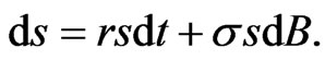
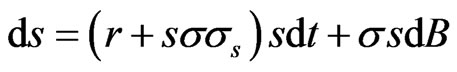
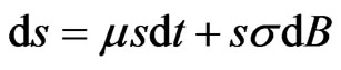
(1)

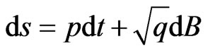
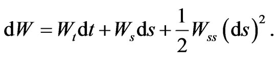
is the process for the risky asset, where is Brownian motion¹, and both may depend on both and Itô’s theorem provides that:

Let denote the riskless rate at time This is generally independent of the stock price by virtue of being riskless.

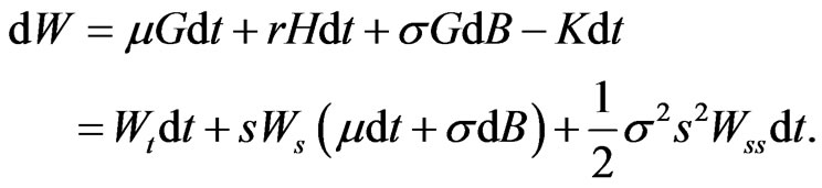
Then, when there are no cash withdrawals or injections (i.e. the strategy is self-financing),

so that

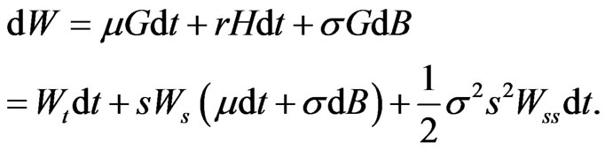(2)

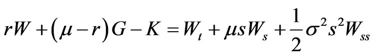
This implies that

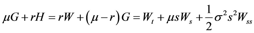(3)

and

(4)

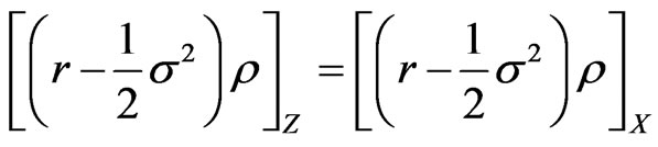
thus

and so

(5)

These equalities are consistent with the conditions of Proposition 1 of [1]. Note that the expected return on the risky asset does not appear in 5.

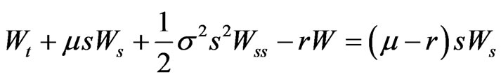
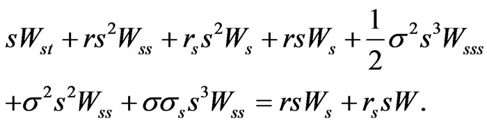
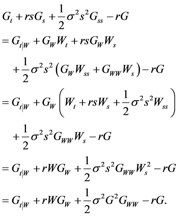
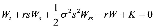
Differentiating equation (5) with respect to yields:

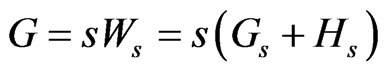
Multiplying this last equality by, we get

On the other hand since we have

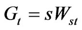
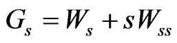
Hence:

and, as this may be formalized as:

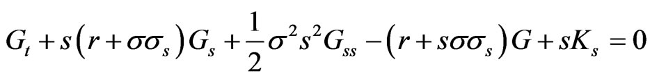
Proposition 1: The controls and satisfy the PDEs:

(6)

(7)

Remark: Thus proposition 1 of [1] will not apply for if However note that has the same form as but with replaced by

3. Controls Based on Wealth

Since we now consider and as functions of This corresponds to Proposition 2 of [1].

On this basis

Hence the left hand side of Equation (7) becomes

For the right hand side of equation (7):

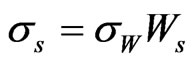
and so

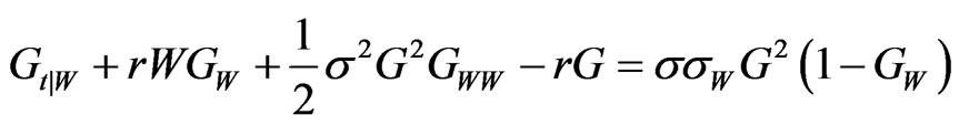
Hence we have:

Proposition 2: The control viewed as a function of wealth, satisfies:

Remark: This is the same as proposition 2 of [1] when

4. Controls That Are Compatible with a Concave Utility

Consider a control that maximizes an expected utility of terminal wealth at time:

for some utility function and where is the physical measure under the process in 1.

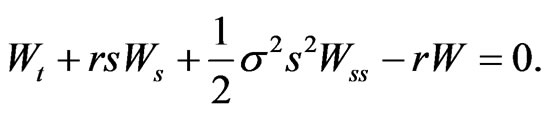
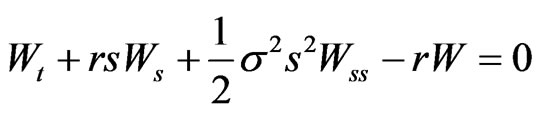
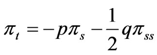
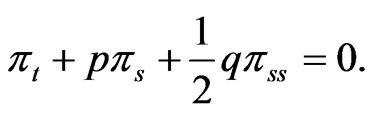
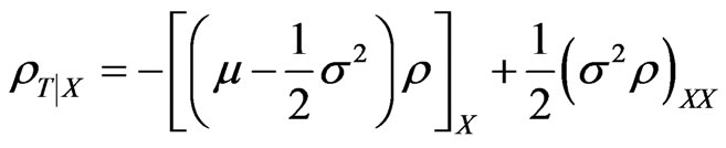
Then the equation (5) is, regarded as a parabolic partial differential equation:

where is a function of and and are functions of.

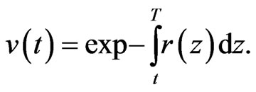
The solution is given by the Feynman-Kac formula. The solution, expressed as a stochastic expectation, is:

(9)

Here and for a given value of and

The expectation is taken with respect to the risk neutral process:

(10)

Remark: It is known there are various conditions for the Feynman-Kac formula to hold, which are set out in the Appendix. A condition that be bounded above zero is not onerous, as we are dealing with a risky asset. Some of these conditions may be relaxed significantly, and will be discussed in a further paper.

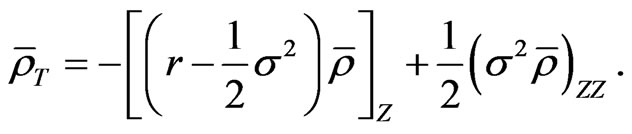
The probability density of at time is governed by the Kolmogorov backward equation

and also the Kolmogorov forward equation

(11)

The conditions for these results are also set out in the Appendix.

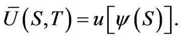
The critical implication of 9 is that and therefore is completely determined by the terminal wealth along with an initial condition, say for some initial stock price

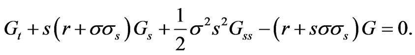
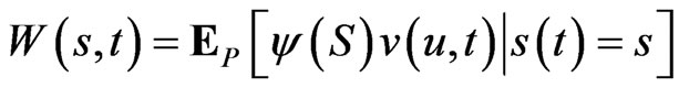
In addition, since satisfies the similar PDE in 7, we have:

(12)

where the expectation is taken with respect to the process:

and

This implies that if

Optimization

Thus for the utility function it suffices to find so as to maximize:

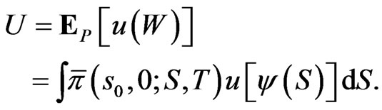
Here the expectation and density relate to the physical stock process:

rather than to 10.

This is subject to the initial condition:

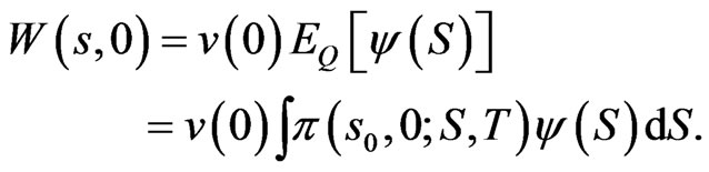
where the expectation is subject to the risk neutral process in 10.

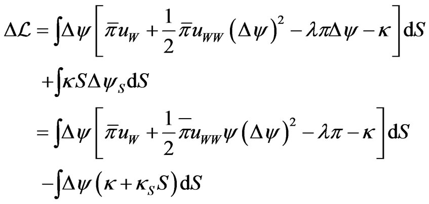
The Lagrangian is

Let be a variation in The resulting variation in is, to the second order:

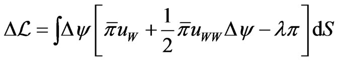
Since for any variations the first order condition is

where Thus given the function may be found from

(14)

with being chosen to satisfy the initial condition 13.

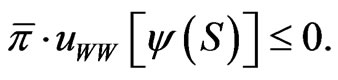
The second order condition is so that a concave utility is required. The general solution for in terms of is then given by 9. In the general case with not constant, we thus have the following extension of the existential results of Proposition 3 of [1]:

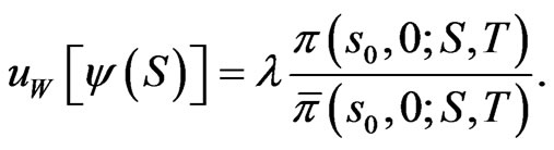
Proposition 3 A path independent strategy can be found to optimize a given concave utility if, and only if, a solution can be found to satisfy:

Remark: This is without qualification as to the existence of a solution to 8. In the case that is given, the Inada conditions provide that is invertible on so that

In the case that is given, the condition is sufficient to determine However none of these conditions is mentioned in Proposition 3 of [1].

Example: [1] assume constant returns and volatilities In this case, it is well known that is normally distributed, with mean

(physical measure) or

(risk neutral measure), and variance at time

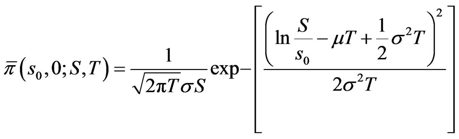
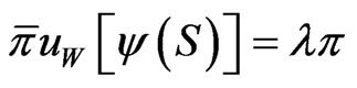
while

Hence 14 becomes:

Differentiating with respect to we also have

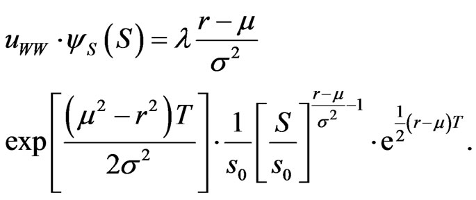
Thus when and vice versa.

By virtue of 12 depending on whether we have a proof of Proposition 3 of [1].

5. Extension of Utility Characterization

It is of interest to consider whether the allocation to the risky asset is non-negative under more general conditions than indicated in Proposition 3 of [1].

Proposition 4 Suppose are non-stochastic (i.e. independent of) and. Then a strategy can be found to optimize a concave utility with

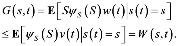
Proof. Given the strategy is given by 14 and the Kac-Feynman formula 9. We also note the relation 12, which shows that if at time

Differentiating 14 with respect to we have:

Since it suffices to show that The variant of Girsanov’s theorem, as proved in the Appendix, confirms this result.

Remark: The conditions are sufficient, but by no means necessary. The Appendix shows that the density of the risk neutral process for

with stochastic is central to this issue. In particular, if the risk premium is non-stochastic, and is concave in then the result also holds. This situation may be investigated by noting that satisfies a parabolic PDE, which can in turn be investigated by the eigenfunctions of the operator

.

6. Constrained Strategies

The above discussion does not constrain the allocations to both the risky asset and the riskless asset to be nonnegative, which is often a requirement in practice. For this to apply, we have the additional constraints on terminal wealth:

If then Proposition 4 provides conditions for To provide that 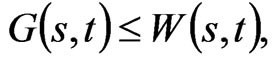we need to have the terminal condition:

(15)

If this holds, and then Equation (12) implies:

To ensure that 15 holds, consider the Lagrangian:

Let be a variation in such that when The variation in is, to the second order:

The first order condition is thus:

which can be written:

and thus integrating over

The second order condition is as before:

This leads to the following result:

Proposition 5: Given a concave utility and the strategy given by the KacFeynman formula 9, provides optimality over nonnegative allocations to the riskless asset, only if there is a solution of:

for some

Remark: These are weaker conditions than provided in Proposition 3, as we are seeking optimality over a smaller class of allocations. Even weaker conditions may be found if the class of allocations is restricted to where both the risky and riskless assets are constrained to be non-negative.

7. Allowance for Cash Flows

The previous relations can be extended to accommodate portfolios with cash withdrawals. Let us now consider the situation when an investor is allowed to withdraw from their investment, at a rate. Such as before, we discuss the cash withdrawn from the portfolio in two cases, a function of price of the risky asset and time, , or a function of total wealth and time,.

Total wealth then obeys the generalised relation:

7.1. Controls That Are Functions of the Value of the Risky Asset and Time

In analogy with section 2 consider the case where the controls, , and, are all functions of, where the process of is the same as in 1.

Allowing for cash withdrawals, 2 generalizes to

(16)

This implies that

(17)

and the same condition as in 4, which is consistent with Proposition 1 of [1] that

and hence 5 generalizes to:

(18)

It may be shown similarly that 7 generalizes to:

(19)

Now we can formalize the above results as:

Proposition 6: Necessary and sufficient conditions for the differentiable functions, and to be the controls of a self-financing investment strategy are that:

(20)

(21)

for all and.

Notice that Proposition 1 of [1] is a special case of this generalized form with a constant diffusion for price of the risky asset, that is.

7.2. Controls That Are Functions of the Value of the Portfolio Wealth and Time

In analogy with section 3, consider the situation when the controls, and, are functions of.

As is a control, we also have:

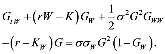
Then Equation (7) can be shown to generalize to:

Proposition 7: The control viewed as a function of wealth, satisfies:

7.3. Compatibility with Investor Objectives

We now consider if the processes of controls and are compatible with rational investor objectives.

Express 18 to get

where, without loss of generality, we write

This is again a parabolic PDE in, and the FeynmanKac formula can be applied to find a solution as:

(23)

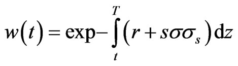
but now the discount factor includes:

As before, the wealth is completely determined by the terminal wealth, along with the control

In the case with cash withdrawals are admissible, we consider not only the utility from terminal wealth for an investor, but also the utility from consumption financed by the cash withdrawals. Therefore, the problem of choosing optimal portfolio and consumption rules for an investor over a period of is to maximize an aggregate utility of the following form:

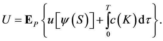
The function is the utility from consumption, with. The initial and terminal times are specified at and, as is the initial condition that some initial stock price. The expectation is specified as before in Section 4 for the physical stock process.

The Lagrangian is then given by:

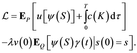
This optimization problem is exactly of continuous stochastic control [20, VII.10]. Define an optimal expected value function given the stock price at time

The process terminates at time, at which time the utility of terminal wealth is assessed, with the boundary condition

(24)

The fundamental PDE for the control is:

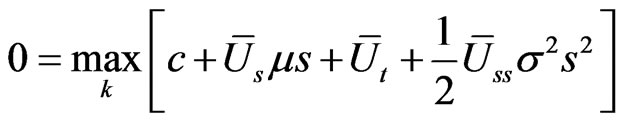(25)

However, we follow an alternative, but simpler, approach. Given consider a small variation in say localized at time and in state

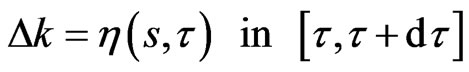
for some constant which induces a variation This further induces variations in the terms

and, to the first order in:

And thus:

Since is localized at and is constant, the first order condition in is:

for some constant

The second order condition in is:

Hence we have the following result.

Proposition 8 Given concave utility functions for terminal wealth and for consumption, and a terminal wealth with density the optimal cash flow control is given by satisfying:

(26)

for some constant

Remark: As is a decreasing function in this implies that cash withdrawals should increase in the wealth achieved, but should decrease where such wealth is less likely to be achieved. This corresponds to the conditions contained in Proposition 4 of [1].

8. Conclusions

In this paper, we address two related issues, based on the work by [1].

First, we examine the characteristics of optimal portfolio controls. Rather than assuming constant expected returns and volatility, we consider the more realistic situation with the expected return and volatility of risky assets are non-constant, or even stochastic.  

Second, we consider whether a given investment strategy is consistent with expected utility maximization. We apply several techniques of the calculus of variations to show that, under mild conditions, optimal portfolio controls are compatible with some concave utility function. Unlike most papers in the literature, we do not specify a particular form of utility function.  

It would be interesting to extend these results to more general asset models, for example where the risky asset follows a jump diffusion process, or where volatility of the return on the risky asset is itself a stochastic process.

REFERENCES

1. Appendix: Conditions for Known Results

Let a general stochastic process be defined by

where and are functions of Let denote the density of at time given an initial value of Derivatives will be taken assuming all other variables are held constant.

We summarize various conditions on and for results to hold. Most of these are cited from [12] and the references therein.

1.1. Conditions

C1 are globally bounded above.

C2 is globally bounded from zero across

C3 and satisfy a global Hölder condition, that is for some parameters and

C4 and satisfy a global Hölder condition with respect to

C5 and the second derivatives with respect to are of most polynomial growth.

C6 are locally Lipschitz.

C7 are of at most linear growth.

C8 is continuous in and locally Lipschitz in

C9 is uniformly bounded and locally Hölder.

1.2. Kolmogorov Forward Equation

The probability density satisfies the Kolmogorov forward equation (11):

This holds under the following conditions [12, Theorem 5.15].

• C1.

• C2.

• C3.

1.3. Kolmogorov Backward Equation

The density 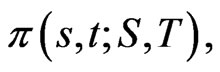considered as a function of also satisfies the Kolmogorov backward equation

This holds under the following conditions [12, Theorem 5.15]:

• C1.

• C2.

1.4. Feynman-Kac Formula

Consider the Equation (5), regarded as a parabolic partial differential equation:

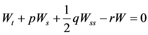(27)

where are functions of as in 5. This is subject to the boundary condition In this section, we allow to be a function of both

The solution is given by the Feynman-Kac formula, expressed as a stochastic expectation:

(28)

where and for a given value of and

The function may be regarded as a generalized discount function for interest.

The Feynman-Kac formula holds under the following conditions:

1) (C5), (C6), (C7) and and and its derivatives are of at most polynomial growth [12, Theorem 6.2].

2) (C7), (C8), (C9) and and is of at most polynomial growth [21, Theorem 5.5].

2. Girsanov’s Theorem

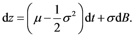
Both the physical process 1 and risk-neutral process 10 for can be simplified under Itô’s lemma by making the transformation Thus in logarithmic terms the physical process can be described by:

and the physical process by:

Where and are non-stochastic, with this provides explicit solutions for the physical and risk neutral densities and in which obey the forward equations:

(29)

and

(30)

For example is normal with mean

and variance Letting and

we have

and thus

(31)

On the other hand the density of the stock price is given by

with so that

Therefore to show that it suffices to show that 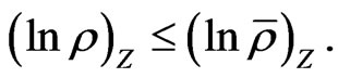This can be shown directly from 31. However we take an approach that illustrates a relationship with Girsanov’s theorem, and allows a generalization to the case where the parameters are stochastic.

Make the transformation 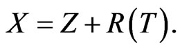We then have

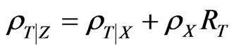
We then have from 29:

Let (so that the risk premium is not stochastic). Then:

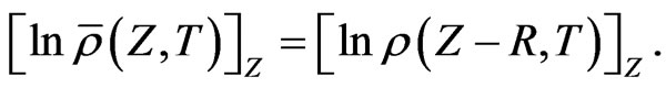
It may be concluded from comparing this equation with 30 that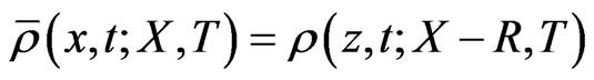, so that changing variables:

If then so that holds if:

This last condition clearly holds in the case of non-stochastic parameters as in 31. However it is a condition on the risk neutral process only, and may hold in other cases where the stock volatility is stochastic.

NOTES

¹We use rather than the more conventional as subscripts in this paper are reserved solely for derivatives.

REFERENCES

- J. C. Cox and H. E. Leland, “On Dynamic Investment Strategies,” Journal of Economic Dynamics and Control, Vol. 24, No. 11-12, 2000, pp. 1859-1880. http://dx.doi.org/10.1016/S0165-1889(99)00095-0
- R. C. Merton, “Optimum Consumption and Portfolio Rules in a Continuoustime Model,” Journal of Economic Theory, Vol. 3, No. 4, 1971, pp. 373-413. http://dx.doi.org/10.1016/0022-0531(71)90038-X
- F. Black and M. Scholes, “The Pricing of Options and Corporate Liabilities,” The Journal of Political Economy, Vol. 81, No. 3, 1973, pp. 637-654. http://dx.doi.org/10.1086/260062
- J. C. Cox and S. A. Ross, “The Valuation of Options for Alternative Stochastic Processes,” Journal of Financial Economics, Vol. 3, No. 1-2, 1976, pp. 145-166. http://dx.doi.org/10.1016/0304-405X(76)90023-4
- P. Carr, H. Geman and D. Madan, “The Fine Structure of Asset Returns: An Empirical Investigation,” Journal of Business, Vol. 75, No. 2, 2002, pp. 305-332. http://dx.doi.org/10.1086/338705
- S. Hodges and R. Clarkson, “Dynamic Asset Allocation: Insights from Theory,” Philosophical Transactions: Physical Sciences and Engineering, Vol. 347, No. 1684, 1994, pp. 587-598.
- R. C. Merton, “Lifetime Consumption under Uncertaintiy: The Continuous Time Case,” The Review of Economics and Statistics, Vol. 51, No. 3, 1969, pp. 247-257. http://dx.doi.org/10.2307/1926560
- S. A. Ross, “Mutual Fund Separation in Financial Theory—The Separating Distributions,” Journal of Economic Theory, Vol. 17, No. 2, 1978, pp. 254-286. http://dx.doi.org/10.1016/0022-0531(78)90073-X
- G. S. Amin and H. M. Kat, “Hedge Fund Performance 1990-2000: Do the ‘Money Machines’ Really Add Value?” Journal of Financial and Quantitative Analysis, Vol. 38, No. 2, 2003, pp. 251-274. http://dx.doi.org/10.2307/4126750
- S. Vanduffel, A. Chernih, M. Maj and W. Schoutens, “A Note on the Suboptimality of Path-Dependent Pay-Offs in Lévy Markets,” Applied Mathematical Finance, Vol. 16, No. 4, 2009, pp. 315-330. http://dx.doi.org/10.1080/13504860802639360
- S. Kassberger and T. Liebmann, “When Are Path-Dependent Payoffs Suboptimal?” 2009.
- F. C. Klebaner, “Introduction to Stochastic Calculus with Applications,” Imperial College Press, London, 2005. http://dx.doi.org/10.1142/p386
- O. C. Ibe, “Markov Processes for Stochastic Modeling,” Elsevier Academic Press, Waltham, 2009.
- M. J. Brennana, E. S. Schwartz and R. Lagnado, “Strategic Asset Allocation,” Journal of Economic Dynamics and Control, Vol. 21, No. 8-9, 1997, pp. 1377-1403. http://dx.doi.org/10.1016/S0165-1889(97)00031-6
- J. Cvitanic and V. Polimenis, “Optimal Portfolio Allocation with Higher Mo Moments,” Annals of Finance, 2008.
- S. P. Sethi, “A note on Mertons Optimum Consumption and Portfolio Rules in a continuous-Time Model,” Journal of Economic Theory, Vol. 46, No. 2, 1988, pp. 395- 401. http://dx.doi.org/10.1016/0022-0531(88)90138-X
- A. Meucci, “Review of Dynamic Allocation Strategies: Utility Maximization, Option Replication, Insurance, Drawdown Control, Convex-Concave Management,” 2010.
- K. Tanaka, “Dynamic Asset Allocation under Stochastic Interest Rate and Market Price of Risk,” 2009.
- C. Chiarella, C. Hsaio and W. Semmler, “Intertemporal Investment Strategies under Inflation Risk,” University of Technology, Sydney, 2007.
- S. E. Dreyfus, “Dynamic Programming and the Calculus of Variations,” Academic Press, Norwell, 1965.
- S. Janson and J. Tysk, “Feynman-Kac Formulas for BlackScholes Type Operators,” Bulletin London Mathematical Society, Vol. 38, No. 2, 2006, pp. 269-282. http://dx.doi.org/10.1112/S0024609306018194