Journal of Mathematical Finance
Vol. 2 No. 4 (2012) , Article ID: 24550 , 12 pages DOI:10.4236/jmf.2012.24032
Closed-Form Approximate Solutions of Window Barrier Options with Term-Structure Volatility and Interest Rates Using the Boundary Integral Method
Department of Finance, National Dong Hwa University, Hualien, Taiwan
Email: hsiao@mail.ndhu.edu.tw
Received August 8, 2012; revised September 10, 2012; accepted September 22, 2012
Keywords: window barrier option; integral method; integral representation; Green’s function; PDE approach
ABSTRACT
In this study we propose an approach to solve a partial differential equation (PDE), the boundary integral method, for the valuation of both discrete and continuous window barrier options, as well as multi-window barrier options within a deterministic term structure of volatility and interest rates. Numerical results reveal that the proposed method yields rapid and highly accurate closed-form approximate solutions. In addition, the term structure will have a significant impact on the valuation.
1. Introduction
Barrier options are widely used and traded in financial markets to manage the risk related to foreign exchange, interest rates, and equity in the global market. A barrier option is a path-dependent option that is activated (i.e. knocked in), or extinguished (i.e. knocked out) when the price of the underlying asset breaches the pre-specified barrier level at any time before maturity. There are two main reasons for the prevalence of barrier options. First, barrier options are useful for limiting the risk exposure of clients, specifically in the foreign exchange market. Second, barrier options are cheaper than vanilla options with similar attributes. Therefore, they are more affordable financial instruments that can match investors’ views regarding the degree of volatility in the underlying asset price change. Additionally, they offer an appropriate level of downside protection for hedging purposes. For example, if long hedgers believe that only a mild volatility exists in the market over a given period, the hedgers will prefer to buy a knock-out option with fewer premiums than to pay the full premium for a plain vanilla option. Alternatively, when speculators believe that the price change will be volatile for a period of time, they will prefer to purchase a knock-in option rather than to obtain the plain option with a higher price. Since an ordinary option can be decomposed into two otherwise identical knock-in and knock-out options, this feature makes the barrier option a highly suitable instrument for tailor-made structured deals.
Partial barrier options are the extension of barrier options, however there is a major difference between the two. Partial barrier options assume that the barrier prevails only for some fraction of the option’s lifetime, while barrier options prevail through the entire life of the option. Heynan and Kat [1] studied two types of continuous partial single barrier options: 1) an option with a monitoring period which commences at the start date of the option and terminates at an arbitrary date before expiration (this is referred to as an early-end partial barrier option); and 2) an option with a monitoring period which commences strictly at the starting date and ends strictly before the expiration date.
A window barrier option incorporates a barrier which commences at an arbitrary date after the starting date and terminates at an arbitrary date before the expiration. Window barrier options are more flexible than standard barrier options because the adaptable monitoring period provides traders with the full flexibility to lock volatility risks during a specific time period. Window barrier options not only offer investors a hedge instrument maneuvered by investors’ views on the range of volatility, but these options also provide building blocks to create various types of partial exotic options embedded in structured products. In recent years they have become more popular with investors, particularly in foreign exchange markets. Meanwhile, academics and practitioners have turned their attention to the more complicated structures of barrier options.
Since Merton [2] first derived the analytical closedform solution to handle a down-and-out continuous monitoring barrier call, there has been a variety of research concerning this issue. Cox and Rubinstein [3] provided a valuation formula for an up-and-out call, which is nullified whenever the underlying asset price triggers the upper knockout price. Rubinstein and Reiner [4] provided the formulae for 8 types of barrier options, and Haug [5] gave a generation of the set of formulae provided by Rubinstein and Reiner. Kunitomo and Ikeda [6] provided valuation formulae based on a generalization of the Levy formula for double barrier options with two exponential curved boundaries. Geman and Yor [7] used the CameronMartin theorem to obtain the Laplace transformation of the values for double barrier options with two fixed boundaries.
The binomial and trinomial lattice models developed respectively by Cox, Ross and Rubinstein [8] and Boyle [9,10] are well-known schemes for pricing standard vanilla options. However, Boyle and Lau [11] demonstrated that the CRR binomial model may lead to persistent errors in barrier option pricing. Ritchken [12] illustrated that when the trinomial model is naively applied to the pricing of barrier options, more time steps may not always lead to more accurate prices. Boyle and Lau [11] and Ritchken [12] suggested modified lattice algorithms to generate accurate pricing for the barrier option. But as revealed in Ritchken [12], the modified algorithms suggested by Boyle and Lau [11] and Ritchken [12] are nevertheless inefficient for handling the barrier-too-close problem. Wang, Liu and Hsiao [13] used a hybrid method, which is a combination of the Laplace transformation and the finite-difference approach, to overcome the unstable problem for pricing barrier options modeled by a branching process. Figlewski and Gao [14] used the adaptive mesh model to discuss option pricing. Albert, Fink, Fink [15] priced barrier options using an adaptive mesh model under a jump-diffusion process.
Broadie, Glasserman, and Kou [16] and Hörfelt [17] derived the approximation formulae for the discrete single barrier options. Boyle and Tian [18] proposed a modified explicit finite difference approach to the valuation of barrier options, but their method is not particularly efficient in dealing with discrete barrier option pricing. Ahn, Figlewski, and Gao [19] suggested the adaptive mesh model structure for pricing discrete barrier options. Kou [20] applied a sequential analysis to extend Broadie, Glasserman and Kou’s approximation formulae [16] to more general cases of discrete barrier options. Mitov, Rachev, Kim and Fabozzi [21] derived an analytical formula for the price of an up-and-out call, and showed that the values of barrier options priced with the branching process in a random environment model were significantly different from those modeled with a lognormal process. Hu and Knessl [22] analyzed the asymptotics of barrier option pricing under the constant elasticity of variance (CEV) process.
Heynen and Kat [1] first derived the closed-form solutions for pricing partial late-start and early-end barrier options under Black-Scholes assumptions [23], and their solutions were expressed in terms of the bivariate normal distribution function. Heynen and Kat [24] extended their closed-form formula to handle a discrete window barrier option where the barrier level may change deterministically and the monitoring points can be of unequal distance to each other. Armstrong [25] extended Heynen and Kat’s closed-form formula [1] and derived formulae with a tripartite deterministic term-structure of interest rates, volatility, and dividend yields in terms of trivariate normal distribution functions. Carr [26] derived a riskneutral expectation formula to value partial barrier options with a constant rebate.
Most of the partial barrier models mentioned previously, with the exception of that of Heynen and Kat [24], assume that the underlying asset is continuously monitored against the partial barrier level. Nevertheless, discrete barrier options are among the most popular time-dependent options traded in markets. In addition, they are monitored discretely only at a particular time, normally, at daily closing (e.g. the capped index spread on the S&P100 and S&P500, and the knock-out barrier options on the All Ordinary Price Index on the Australian Stock Exchange). Although Chance [27], Kat and Verdonk [28] indicated that there exists a substantial price difference between barrier options and their otherwise identical continuous counterparts even under daily monitoring, the exact pricing formula was still not extended to discrete window barrier options with more complex features such as a varying rebate, barrier, and volatility with a discrete monitoring period.
This paper proposes the boundary integral method (BIM) [29], which is an efficient partial differential equation (PDE) approach, to price both continuous and discrete window barrier options under the Black-Scholes economy. We extend the continuous models of Heynen and Kat [1] and Armstrong [25] to include time-dependent rebates and a tripartite deterministic term structure of interest rates and volatility. In addition, the BIM can easily be further extended to the valuation of multiwindow barrier options characterized with a ladder strike prices. The discrete window barrier option of Heynen and Kat [24] is also extended to accommodate the multipartite term structure of interest rates and volatility. We also demonstrate that the proposed integral method is capable of valuating the discrete window double barrier option. Numerical examples and comparisons with Armstrong [25] confirm that the BIM will yield rapid and highly accurate numerical solutions for both discrete and continuous window barrier options. In addition, the numerical examples confirm that the BIM has a convergence rate of order 4 in the case of discrete window barrier option pricing.
This paper is organized as follows: in Section 2 we present the valuation algorithm in terms of the initial value problem and boundary value problem. We also explain how to deal with discontinuities caused by the window barrier feature, and demonstrate how to recursively obtain the option price. Section 3 discusses the valuation of discrete window barrier options, and defines the pricing problem as a sequence of the initial value problem. Section 4 contains numerical results, and Section 5 concludes with a summary and some suggestions for future research.
2. Methodology
2.1. Preliminary Assumptions
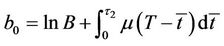
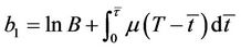
Since a knock-in window barrier option plus a knock-out window barrier option will be equal to the value of an otherwise equivalent vanilla option, we will concentrate only on the knock-out window barrier option. Let 0, t1, t2, and T denote the option’s starting date, the time to the start of the barrier, the time to the end of the barrier, and the option’s maturity date, respectively, and 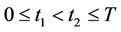 . The valuation of the early-ending window barrier option can be calculated by letting t1 approach 0, and the valuation of the forward-start window barrier option can be recovered by letting t2 approach T.
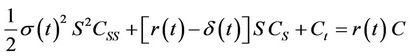
Our objective is to apply the PDE (partial differential equation) approach to the valuation of the window barrier option in Black-Scholes economy assumptions. When the underlying is assumed to follow a lognormal random walk, under no arbitrage argument, the PDE governing the window barrier option will be as follows:
 , (1)
, (1)
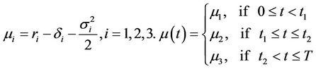
where C is the option value, S is the underlying asset price,  is stock’s volatility,
  is the risk-free interest rate,
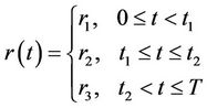
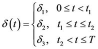
  is the dividend yield, and t is the time. To allow for the case of greatest generality, the stock’s volatility and the risk-free interest rate may change deterministically across the barrier monitoring period. We allow for three different governing PDEs, or we may say, the Black-Scholes equation with different coefficients for time intervals [0, t1), [t1, t2], and (t2, T]. As in Armstrong [25], we assume a simple tripartite term structure that naturally accommodates the location of the barrier, and the risk-free interest rate, dividend yield, and volatility are given by the following step functions:
 ,
,
 ,
,
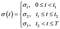 .
.
When the underlying asset price does not touch or breach the barrier level through the monitoring period, the payoff of the window barrier option at the maturity date is given as the following equation:
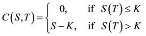 , (2)
, (2)
where K denotes the strike price.
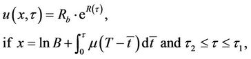
Oppositely, if the underlying asset price triggers the barrier level throughout the monitoring period, the option will be knocked out and clients will receive an immediate rebate Rb. The payoff is as follows:
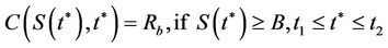 (3)
(3)
where B denotes the barrier price and Rb denotes the immediate rebate.
The equation (1) is the governing equation and conditions (2) and (3) are the initial condition and boundary condition for the call price C(S, t) respectively.
Let
Making the following variable transformations:
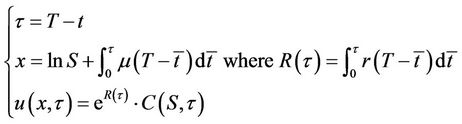 , (4)
, (4)
equation (1) can be simplified into the heat equation with a constant diffusion coefficient as follows:
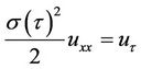 (5)
(5)
The payoff of the window barrier option at the maturity date  will be transformed into:
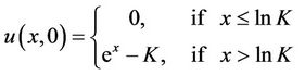 . (6)
. (6)
Since the asset price is assumed to change continuously with time, if the asset price S(τ) breaches the barrier level between time interval , it will first touch the barrier level. Therefore the payoff of the option can be transformed, as in equation (7).
 (7)
(7)
where  and
and .
.
2.2. Boundary Integral Method
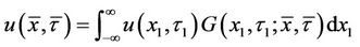
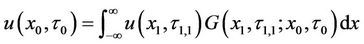
On the time interval , there is not any boundary condition; hence the solution of the PDE is uniquely determined by the initial condition (6). The problem of finding the unique solution with PDE (5) and initial condition (6) is termed the initial value problem. In our notation, the integral representation of the solution will be:
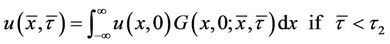 (8)
(8)
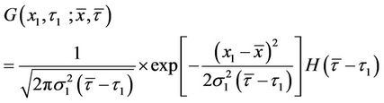
where the function G is called Green’s function with the infinite domain or the fundamental solution of the heat equation. It can be expressed as follows:
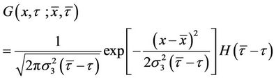 , (9)
, (9)
where  is the Heaviside step function, and is defined by:
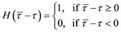 . (10)
Equation (8) has some interesting interpretations with respect to the risk-neutral approach of Cox and Rubinstein [3].  and Green’s function can be interpreted as the option’s terminal payoff and its risk-neutral probability density function, respectively. Thus the integral representation of the solution can be interpreted as the option’s expected terminal payoff, and the value of the window barrier option at time
  will be equal to its discounted expected value as suggested by equation (4).
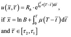
As in Black-Scholes [23], equation (8) can be further simplified into a closed-form solution as:
 , (11)
where N (.) is the cumulative normal distribution function. 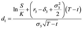 and
and
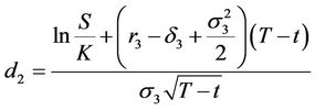 .
.
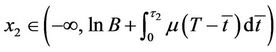
However, if the transformed underlying asset price x2 is within the range 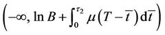 at
at the instant after it passes the monitoring date, i.e.
 , the transformed window barrier price will still change continuously across the barrier monitoring date
 . If we denote
  as the instant after
 , the continuity assumption will guarantee that
  will be equal to
 . Therefore, the initial condition for equation (5) between
  will be as follows:
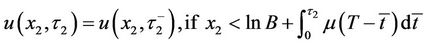 ,(12)
,(12)
where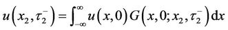 .
.
If the underlying asset price breaches the barrier level during the period, the window barrier option will be knocked out, and clients will receive an immediate rebate Rb. The continuity property will guarantee that the asset price first touches the barrier level before it breaches the barrier level. Thus, the boundary condition for Equation (5) between  will be specified as in Equation (13):
 . (13)
There exists only one solution that satisfies the PDE (5) and is subject to the initial condition (12) and the boundary condition (13). The integral representation of a solution for the heat equation at  is as follows:
If , and
, and , then
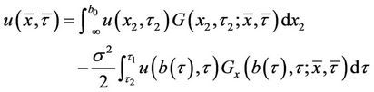 , (14)
where 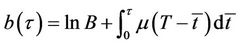 and
and
 .
.
G is the green function with the boundary .
.
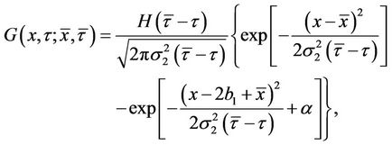
where b1 is the transformed barrier price at ,
,  ,
, 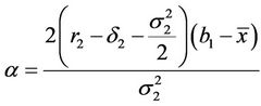 and
and
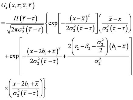 . (15)
The functions G(.) and Gx(.) in equation (14) can be interpreted as the transition probability density function and the hitting probability density function of the transformed underlying asset price, respectively. The first term in equation (14) is the expected payoff when the barrier is never breached throughout the monitoring interval [ ,
, ], and the second term is the expected payoff when the underlying asset price breaches the barrier in the time interval [
 ,
, ]. Once again the solution can be interpreted as the expected payoff in a risk-neutral environment.
Finally, we will discuss how to cope with parameter discontinuities and obtain the ultimate solution  . Let
. Let  denote the instant after
 ; the parameter discontinuity happening between time to maturity
  and
and  can be overcome with the same logic as in equation (12). That is, when
  approaches
 ,
,  will be equal to
 . The solution problem once again is an initial value problem analogous to the first period valuation from
  to
to . Therefore the initial condition for differential equation (5) between time interval
  has to be
 , and the integral representation of the closed-form approximate solution for
  is as follows:
 , (16)
where Green’s function is denoted by equation (17),
 . (17)
Finally, the theoretical value for the window barrier option,  , can easily be obtained by the following inverse transformation:
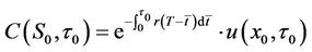 , (18)
where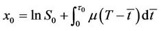 .
.
A key benefit of adopting the PDE approach is that it reduces the pricing problem for the window barrier option to two initial value problems and one boundary value problem, for all of which standard mathematical engineering numerical algorithms are well developed. These algorithms allow a straightforward numerical integration of highly accurate numerical values for window barrier options pricing. Since the Black-Scholes equation can be simplified into a homogenous linear equation such as the heat equation, the boundary integral method proposed in this paper will be a highly efficient algorithm to calculate window barrier options’ numerical solution.
In brief, the valuation of the standard partial barrier call can be divided into a three-phase process, as demonstrated in Figure 1. In the first phase, the terminal payoff at the maturity date,  is the initial condition for the PDE at
 . By applying the integral method, we calculate the convolution of the initial condition
  and Green’s function to acquire the integral representation of numerical solution
  at
at . Next, although the parameter discontinuity caused by the window barrier features will occur at
 , the instant after the monitoring date
 , if
, if
 ,
,  has to be continuous at
 . Thus the parameter discontinuity at
  can be handled accordingly, and the initial condition and the boundary condition imposing on the heat equation can be denoted as in equations (12) and (13). Since the Green function under such boundary constraints exists and is available, the boundary integral method can be applied to acquire the unique solution for differential equation (5) at time to maturity
 . In the third phase, the discontinuity problem between
  and
and  can be handled in the same manner as in phase 2. Thus
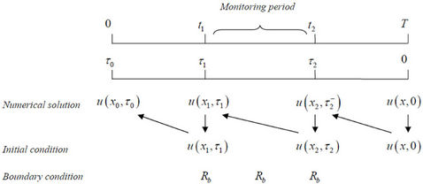
Figure 1. Three-phase process on solving the pricing of the window barrier option. Note: ;
;  = the option’s starting date; 0 = the option’s maturity date;
  to
to  = the option’s monitoring period.
 will be the initial condition imposing on the differential equation between
 . Hence, the problem of finding
  will be an initial value problem again, and the integral representation of the solution can be obtained easily, as in phase 1. The transformation of
  by Equation (18) will ultimately obtain the numerical solution of the window barrier option
 . In Equations (8), (14) and (16), u(.) and G(.) are very smooth functions. Thus, a simple integration scheme such as the Simpson integral will obtain exceptionally precise closed-form approximate values for both
  and
and . Finally, a highly accurate estimation of
  can be obtained by recursively integrating backward through time.
The boundary integral method proposed in this paper can be easily extended to a multi-window barrier option or window ladder option. It also accommodates the pricing of early-end and late-start barrier options. The extra flexibility makes the proposed method an applicable way to calculate options with more complex features. Figure 1 schematically explains the concept of a recursive algorithm. Since the parameter settings, the initial condition, and the boundary condition can be manipulated easily in a standard setting, the recursive algorithm can provide flexibility to tailor a barrier position, duration, barrier level, rebate, and strike price between monitoring periods, so as to suit investors’ unique needs. It can also accommodate multi-partite term structure interest rates and volatility.
3. Recursive Integral Method
In practice, barrier options are frequently monitored only at specific discrete dates. The discrete feature will cause a knock-out window barrier option to be more expensive and a knock-in window barrier option to be less expensive than their respective continuous monitoring counterparts. In this section, we still assume the Black-Scholes economy, but it is not necessary to assume a flat term-structure and constant volatility. As in the pricing of a continuous window barrier option, the term-structure interest rates and volatility can be multi-partite step functions that accommodate the location of the discrete barrier. The PDE approach also allows that the discrete barrier level may change deterministically during the monitoring period, and monitoring need not necessarily take place at equal-spaced points in time. Since the multipartite term structure of interest rates and volatility can be easily handled in the standard setting, for the purpose of simplifying the notations and focusing on the main idea of the recursive integral method, we will assume constant volatility and a flat term structure in this section.
Assume the option monitoring period [t1, t2] is partitioned into m − 1 discrete time intervals, and the option is subject to m times of discrete monitoring. If 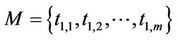 denotes the set of discrete monitoring date, and
  is for the corresponding set of time to maturity. In addition, we assume that the relations between the discrete monitoring dates are
 ,
,  .
.
 denotes the instant after the corresponding discrete monitoring dates.
Under these assumptions, equation (6) is still the initial condition for differential equation (5) between , and
, and  is still the unique solution that satisfies the differential equation (5) at
  subject to the initial condition (6). Since no monitoring is required during time interval
 , the mathematical problem of finding the solution for difference equation (5) at
  will be simplified to become an initial value problem. The solution
  that satisfies the partial differential equation (5) subject to initial condition (6) will be as follows:
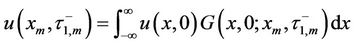 . (19)
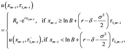
The discrete monitoring feature will introduce m discontinuities into solutions at discrete monitoring dates M*. Following the same logic as discussed in the section on pricing a continuous window barrier option, the instant after the discrete monitoring date  if
if
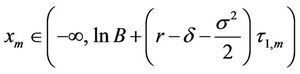 , the value of the window barrier option will change continuously across the discrete monitoring date
 , thus
  will be equal to
 . Otherwise, it will be equal to
  according to the pre-specified contract rebate specification. Thus the solution
  can be defined as follows:
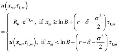 . (20)
Equation (20) will be the initial condition for Equation (5) between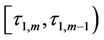 , and the unique solution for equation (5) at
  is given by equation (21).
 (21)
(21)
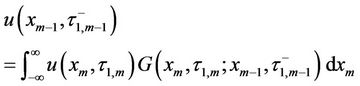
By applying the same argument, the integral representations of solutions for differential equation (5) at ,
,  ,
,  , are given by the recursive integral method as follows:
 (22)
(22)
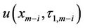
for .
.
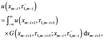
 (23)
(23)
for .
.
Finally,  will be equal to
  as in the continuous window barrier option case in Section 2, and
  can be obtained by using
  as the initial condition, and the unique solution for equation (5) subject to initial condition
  will be:
 , (24)
and  can be obtained by dividing
  with
with  as specified in equation (4).
The valuation of the discrete window barrier option can be defined as a sequence of initial value problems. The proposed recursive integral method is quite analogous to the lattice models and finite difference algorithm. All approaches involve the initial value and work backward to find a solution one step back in time, but there are no intermediate time steps between two discrete monitoring dates for the integral approach. The key advantage of the PDE approach is that most of the standard techniques for solving the PDE in engineering mathematics can be applied to calculate the option pricing, and it can provide practitioners with a more flexible and applicable way to accommodate the complexities of OTC exotic options. Furthermore, when the composite Simpson’s rule is applied to estimate the numerical solution of , Wang and Hsiao [30] prove that the recursive integral method will have a convergence rate of order 4. Hence, the proposed recursive integral method will easily obtain a rapid and highly accurate solution for the discrete window barrier option.
4. Numerical Examples
This section provides some numerical examples, and studies the performance of the BIM algorithm for different choices of parameter settings. To assess the validity of our approach, we compare our continuous window barrier option results with numerical results presented in Armstrong [25], and the parameter settings of the discrete window barrier option is identical to numerical examples discussed in Heynen and Kat [24].
Table 1 investigates the convergence rate of the BIM under different assumptions of stock prices. All examples demonstrate that the BIM has approximately a convergence rate of order 2. When the region of integration in the equation is partitioned into only 128 subintervals, the precision of our valuation algorithm has reached at least a 5 significant digit level in all cases. Table 2 examines the impact of the “barrier-too-close” upon the validity of our proposed algorithm. All numerical examples still demonstrate that the BIM has approximately a convergence rate of order 2, and highly precise numerical values can be easily obtained with the region of integration partitioned into only 128 subintervals. Since we do not partition the underlying asset and time into node spaces as in lattice models, there is no discretization error or approximation error. Numerical examples in Table 2 confirm that the BIM will not encounter the “barrierto-close” problem in the pricing of window barrier options.
Table 3 compares our numerical results with Armstrong’s [25] valuation formula under constant and tripartite term structure scenarios. Its parameter settings are identical to those found in Table 1 from Armstrong [25]. The BIM reveals an excellent rate of convergence in all six examples. If we round the numerical solutions to the nearest integer as in Armstrong’s examples, the numerical values in 5 out of 6 examples will rapidly converge identically to Armstrong’s results for only 32 subintervals in the region of integration1.
Table 4 reports prices of a discrete window down-andout call using the recursive integral method presented in this paper. The option parameters used are identical to those in Heynen and Kat [24]2. Table 4 shows that the recursive integral method has approximately a convergence rate of order 4 as proven in Wang and Shen [29], and the numerical solution will have a precision of up to 10−4 with only 64 subintervals.
To assess the impact of the discrete feature upon the pricing of window barrier option, Table 5 reports the pricing of a discrete window barrier option by using the window barrier option parameter settings as in Table 3, scenario A. Table 5 reveals that the value of discrete
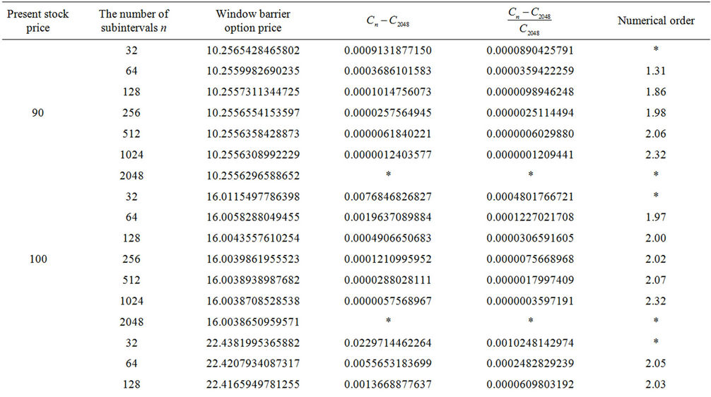
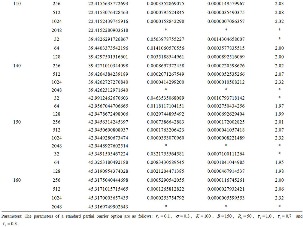
Table 1. Convergence rate for the integral method at various numbers of subintervals.
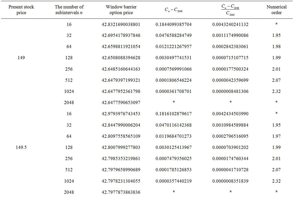
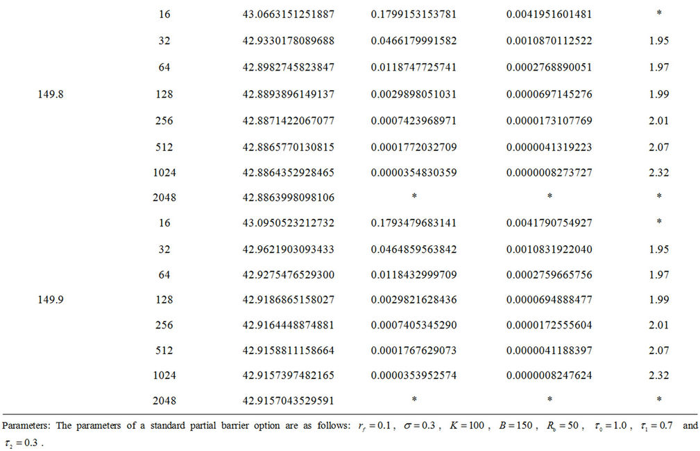
Table 2. Convergence rate for the integral method at various numbers of subintervals.
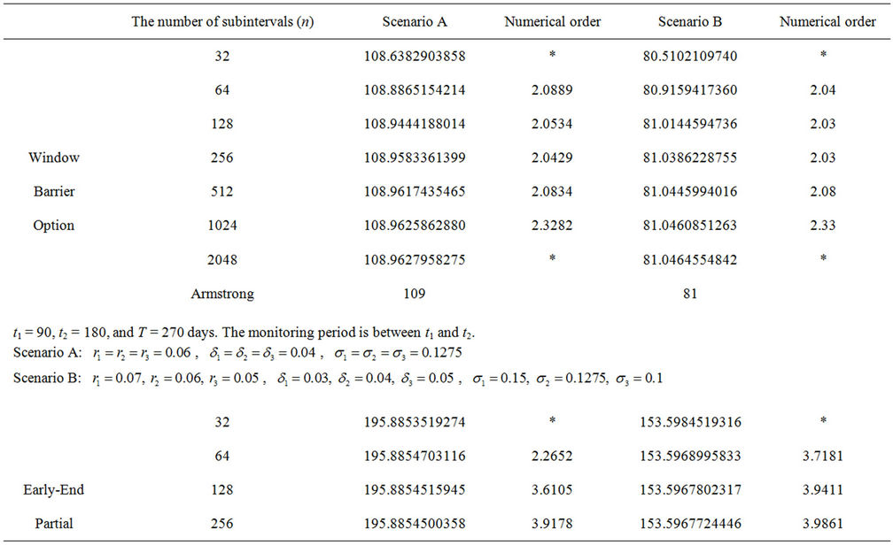
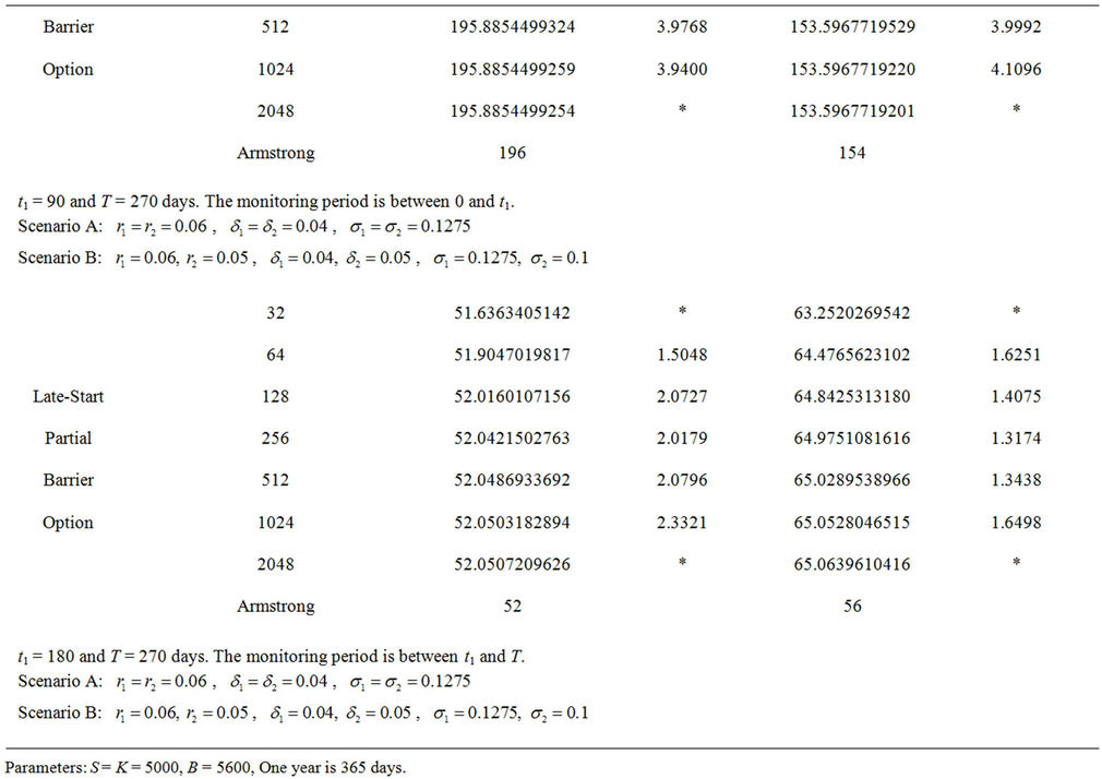
Table 3. A comparison with Armstrong’s approach.
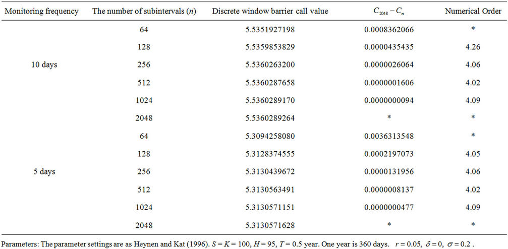
Table 4. Valuation of discrete window barrier down-and-out call.
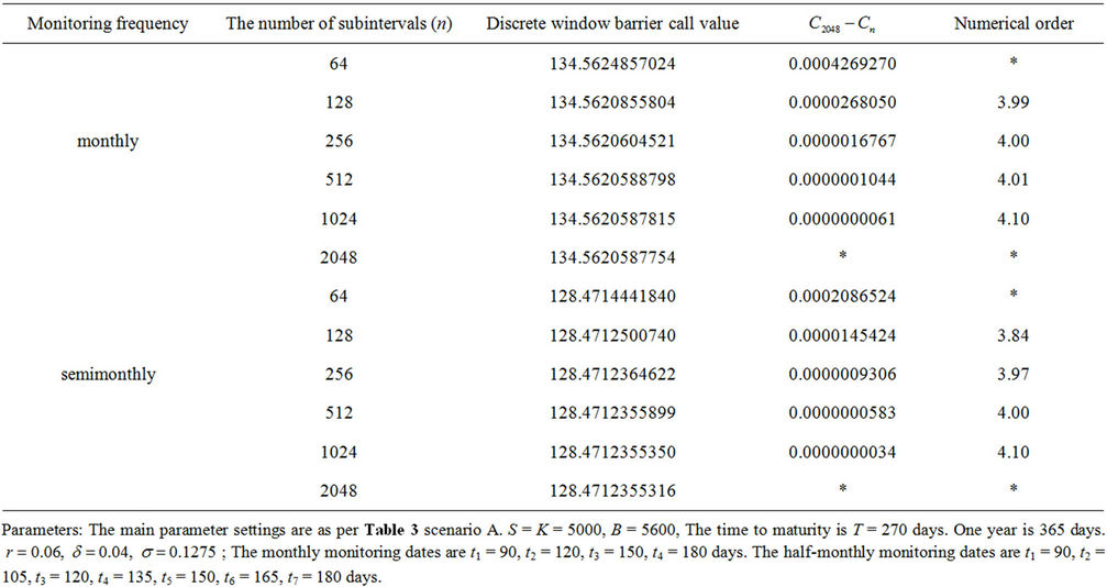
Table 5. Valuation of discrete window barrier up-and-out call.
window barrier option is significantly more than its continuous counterpart, and the difference is negatively related to the frequency of discrete monitoring.
5. Conclusion and Further Research
We have proposed a PDE approach, the boundary integral method, to the valuation of discrete and continuous window barrier options. Numerical examples reveal that the BIM can rapidly obtain highly accurate closed-form approximate solutions for both types of window barrier options, and the term structure can have a significant impact on the pricing of both discrete and continuous window barrier options. The proposed algorithm can provide flexibility to tailor the barrier position, duration, cured barrier, varying rebates, monitoring frequencies, and varying strike prices to suit investors’ unique needs. The extra flexibility offered by the BIM makes it an applicable way to calculate options with more complex features. The BIM is able to easily handle the valuation of a multi-window barrier option by repeating the recursive integral procedures. In addition, it can cope with a discrete window double barrier option by changing the definition of the initial condition accordingly. The proposed PDE approach can also be extended to the Boundary Element Method to accommodate a continuous window double barrier option with cured boundaries.
REFERENCES
- R. Heynen and H. Kat, “Partial barrier options,” Journal of Financial Engineering, Vol. 3, No. 4, 1994, pp. 253- 274.
- R. C. Merton, “Theory of Rational Option Pricing,” Bell Journal of Economics and Management Science, Vol. 4, No. 1, 1973, pp. 141-183. doi:10.2307/3003143
- J. C. Cox and M. Rubinstein, “Options Markets,” Prentice-Hall, Upper Saddle River, 1985.
- M. Rubinstein and E. Reiner, “Breaking Down the Barriers,” RISK, Vol. 4, No. 8, 1991, pp. 28-35.
- E. Haug, “The Complete Guide to Option Pricing Formulas,” McGraw Hill, New York, 1997.
- N. Kunitomo and M. Ikeda, “Pricing Options with Curved Boundaries,” Mathematical Finance, Vol. 2, No. 4, 1992, pp. 275-298. doi:10.1111/j.1467-9965.1992.tb00033.x
- H. Geman and M. Yor, “Pricing and Hedging Double- Barrier Options: A Probabilistic Approach,” Mathematical Finance, Vol. 6, No. 4, 1996, pp. 365-378. doi:10.1111/j.1467-9965.1996.tb00122.x
- J. C. Cox, S. A. Ross and M. Rubinstein, “Option Pricing: A Simplified Approach,” Journal of Financial Economics, Vol. 7, No. 3, 1979, pp. 229-264. doi:10.1016/0304-405X(79)90015-1
- P. P. Boyle, “Option Valuation Using a Three-Jump Process,” International Options Journal, Vol. 3, 1986, pp. 7- 12.
- P. P. Boyle, “A Lattice Framework for Option Pricing with Two State Variables,” Journal of Financial and Quantitative Analysis, Vol. 23, No. 1, 1988, pp. 1-12. doi:10.2307/2331019
- P. P. Boyle and S. H. Lau, “Bumping up against the Barrier with the Binomial Method,” Journal of Derivatives, Vol. 1, No. 4, 1994, pp. 6-14. doi:10.3905/jod.1994.407891
- P. Ritchken, “On Pricing Barrier Options,” Journal of Derivatives, Vol. 3, No. 2, 1995, pp. 19-28. doi:10.3905/jod.1995.407939
- M. L. Wang, Y. H. Liu and Y. L. Hsiao, “Barrier Option Pricing: A Hybrid Method Approach,” Quantitative Finance, Vol. 9, No. 3, 2009, pp. 341-352. doi:10.1080/14697680802595593
- S. Figlewski and B. Gao, “The Adaptive Mesh Model: A New Approach to Efficient Option Pricing,” Journal of Financial Economics, Vol. 53, No. 3, 1999, pp. 313-351. doi:10.1016/S0304-405X(99)00024-0
- M. Albert, J. Fink and K. E. Fink, “Adaptive Mesh Modeling and Barrier Option Pricing under a Jump-Diffusion Process,” Journal of Financial Research, Vol. 31, No. 4, 2008, pp. 381-408. doi:10.1111/j.1475-6803.2008.00244.x
- M. Broadie, P. Glasserman and S. Kuo, “Connecting Discrete and Continuous Path-Dependent Options,” Finance and Stochastics, Vol. 3, No. 1, 1999, pp. 55-82. doi:10.1007/s007800050052
- P. Hörfelt, “Extension of the Corrected Barrier Approximation by Broadie, Glassman, and Kou,” Finance and Stochastics, Vol. 7, 2003, pp. 231-243. doi:10.1007/s007800200077
- P. P. Boyle and Y. Tian, “An Explicit Finite Difference Approach to the Pricing of Barrier Options,” Journal Applied Mathematical Finance, Vol. 5, No. 1, 1998, pp. 17- 43. doi:10.1080/135048698334718
- D. Ahn, S. Figlewski and B. Gao, “Pricing Discrete Barrier Options with an Adaptive Mesh Model,” Journal of Derivatives, Vol. 6, No. 4, 1999, pp. 33-43. doi:10.3905/jod.1999.319127
- S. G. Kou, “On Pricing of Discrete Barrier Options,” Statistica Sinica, Vol. 13, No. 4, 2003, pp. 955-964.
- G. K. Mitov, S. T. Rachev, Y. S. Kim and F. J. Fabozzi, “Barrier Option Pricing by Branching Processes,” International Journal of Theoretical and Applied Finance, Vol. 12, No. 7, 2009, pp. 1055-1073. doi:10.1142/S0219024909005555
- F. Hu and C. Knessl, “Asymptotics of Barrier Option Pricing under the CEV Process,” Applied Mathematical Finance, Vol. 17, No. 3, 2010, pp. 261-300. doi:10.1080/13504860903335355
- F. Black and M. Scholes, “The Pricing of Options and Corporate Liabilities,” Journal of Political Economy, Vol. 81, No. 3, 1973, pp. 637-659. doi:10.1086/260062
- R. Heynen and H. Kat, “Discrete Partial Barrier Options with a Moving Barrier,” Journal of Financial Engineering, Vol. 5, No. 3, 1996, pp. 199-209.
- G. F. Armstrong, “Valuation Formulae for Window Barrier Options,” Applied Mathematical Finance, Vol. 8, No. 4, 2001, pp. 197-208. doi:10.1080/13504860210124607
- P. Carr, “Two Extensions to Barrier Option Valuation,” Applied Mathematical Finance, Vol. 2, No. 3, 1995, pp. 173-209. doi:10.1080/13504869500000010
- D. Chance, “The Pricing and Hedging of Limited Exercise Caps and Spreads,” Journal of Financial Research, Vol. 17, No. 4, 1994, pp. 561-584.
- H. Kat and L. Verdonk, “Tree Surgery,” RISK, Vol. 8, No. 2, 1995, pp. 53-56.
- M. L. Wang and S. Y. Shen, “On Pricing of the Up-andOut Call—A Boundary Integral Method Approach,” Asia Pacific Management Review, Vol. 10, No. 3, 2005, pp. 205-213.
- M. L. Wang and Y. L. Hsiao, “A PDE Approach to Valuation of Discrete Barrier Option,” Working Paper, 2012.
NOTES
1In Armstrong [25], the value of late-start partial barrier option is equal to 56 instead of 65 under scenario B. Since Armstrong did not clearly specify parameter settings for the late-start partial barrier option, we have tried different combinations of parameter settings, and found that the parameter settings we used are consistent with other examples, and should be the most likely settings. We suspect that Typing error may exist in Armstrong’s examples.
2Since Heynen and Kat [24] only present a figure for discrete down-and-out call, we can not directly compare our numerical results. However, the option premiums inferred from the figure is highly similar to our results.