Journal of Mathematical Finance
Vol.2 No.3(2012), Article ID:22117,13 pages DOI:10.4236/jmf.2012.23025
Crisis, Value at Risk and Conditional Extreme Value Theory via the NIG + Jump Model
Department of Finance and Decision Sciences, Hong Kong Baptist University, Hong Kong, China
Email: symzeto@hkbu.edu.hk
Received May 21, 2012; revised June 23, 2012; accepted July 2, 2012
Keywords: Value-at-Risk; Extreme Value Theory; Jump; NIG
ABSTRACT
This study develops a new conditional extreme value theory-based model (EVT) combined with the NIG + Jump model to forecast extreme risks. This paper utilizes the NIG + Jump model to asymmetrically feedback the past realization of jump innovation to the future volatility of the return distribution and uses the EVT to model the tail distribution of the NIG + Jump-processed residuals. The model is compared to the GARCH-t model and NIG + Jump model to evaluate its performance in estimating extreme losses in three major market crashes and crises. The results show that the conditional EVT-NIG + Jump model outperforms the GARCH and GARCH-t models in depicting the non-normality and in providing accurate VaR forecasts in the in-sample and out-sample tests. The EVT-NIG + Jump model, which can measure the volatility of extreme price movement in capital markets due to unexpected events, enhances the EVT-based model for measuring the tail risk.
1. Introduction
Along with the Asian financial crisis of 1997 that caused severe slumps of currencies and the devaluation of stock markets in Asian countries, the global financial crisis that occurred in 2007 represents one of the serious financial crises that triggered extreme volatility in capital markets of both developed and developing countries. It led to the collapse of banks, financial institutions and conglomerates, bringing serious loss to creditors and investors. In response to these events, regulators have become more concerned about the protection of financial institutions against these catastrophic market risks. Value-at-Risk (VaR) has become a standard measure for risk management, yet it is well known that the distributions of the return series in most financial markets are heavily tailed. Traditional risk measuring models such as Riskmetrics focus on the whole distribution and fail to provide an accurate measure of extreme price movements. Additionally, the traditional VaR method has been criticized for violating the requirement of subadditivity [1,2].
To account for the heavily tailed distribution in financial returns, researchers have extensively derived and modified VaR models. Most researchers have developed VaR models that incorporate either asymmetric distributions or the extreme value theory. For instance, Bali and Theodossiou [3] derived a conditional VaR with a skewed generalized t.
Longin [4] proposed considering the estimation of capital requirements as a problem of extreme value calculation. Longin also presented an approach for computing VaR using the EVT model. The parametric extreme value method that focuses on the extreme tails of the distribution allows for an extension of the curve beyond the range of data [5]. This allows the EVT model to estimate extreme losses better than classical methods that use normal distributions [6]. The unconditional EVT has been applied to measure the downside risk in equity markets [7].
Bali [8] also introduced a generalized extreme value approach to financial risk measurement. Bali [9] tested an asymptotic distribution for extreme changes in US Treasury yields and showed that the extreme value approach provided a more accurate estimation of VaR than standard models. Bali and Neftci [10] developed a conditional approach to derive VaR by specifying the location and scale parameters of the generalized Pareto distribution (GPD) as a function of past information, which was found to provide an accurate forecast of the occurrence and size of extreme observations. The EVT has been commonly applied in both financial and insurance risk management [11-13]. Bali [8] proposed a Box-Cox generalized extreme value distribution model to capture extreme events in financial markets.
Although the unconditional EVT approach provides asymptotic results in the distribution of extreme loss for long-term investment decisions, the primary concern for a risk manager is the possibility of loss due to adversarial market movement during the next couple of days, where the dynamics of the time-varying volatility are important. Hence, it seems more appropriate to use the conditional EVT method when estimating day-to-day risk exposures and short-term risk management [14].
Smith [15] suggested an approach to deal with stochastic volatility via a change-point model for extreme value parameters. McNeil and Frey [16] attempted to estimate VaR by incorporating the GARCH model with threshold-based EVT tools, while Byström [14] modified the approach by creating a conditional VaR estimate using the block maxima method. Their conditional models corrected the clustering of extreme events due to stochastic volatility. The models were able to capture the dynamics of the current volatility better than the unconditional model [16]. Bali and Weinbaum [17] introduced a daily conditional extreme value volatility estimator in view of the significant persistence in the parameters for a GEV distribution of high frequency returns within a fixed time interval. Approaches for VaR estimation that use GPD and empirical distribution functions to model tail events and to capture normal market conditions, respectively, have been proposed by some researchers [18].
Byström [14] used both the block maxima approach and the threshold approach in estimating conditional VaR and found that the two models performed similarly. Hence, this study was extended to create the conditional VaR by first using the regime switching model to construct the conditional volatility of the distribution. Then, the EVT model using the threshold method was employed to estimate the distribution of the residuals. In 1982, Engle [19] proposed the autoregressive conditionally heteroskedastic (ARCH) model in estimating market volatility. Subsequently, the GARCH model was developed by Bollerslev [20] and Taylor [21]. Variations and enhancements of the GARCH models have been substantially generated by researchers. It is, however, indicated that extreme declines in the price in securities markets due to unexpected events like stock market crashes or financial crises cannot be fully explained by these GARCH models [22]. Researchers such as Maheu and McCurdy [23] demonstrated that these unusual events may be better captured by jumps.
Maheu and McCurdy [23] proposed a GARCH model that incorporated a heterogeneous Poisson process with a conditional intensity parameter to govern the occurrence of jumps. Maheu and McCurdy [23] explained that the news process is divided into two components: normal news and unusual news events. Normal news innovations cause changes in the conditional variance of returns. The second component of the news process, however, leads to sudden jumps in price over a very short period of time that could be better captured by jumps rather than Brownian motion. Hence, this model captures the excess volatility resulting from unexpected changes in the financial time series.
The motivation of this paper is to propose a model (the EVT-NIG + Jump model) that further enhances the performance of the VaR model in capturing extreme losses by incorporating the NIG + Jump model with EVT and to compare its performance with seven other models in VaR forecasting. This paper focuses on the study of negative tails and examines the fitting and forecasting performance of the models when they are applied to a series of market crashes and financial crises. This study examines whether the proposed VaR models can better forecast the burst of market bubbles. The study focuses on three major crises: the Asian Financial Crisis (AFC) in 1997, the Dot-Com Bubble (DCB) burst in 2000 and the Global Financial Crisis (GFS) in 2007. The AFC was triggered by a financial overextension of the Thailand economy that led to the subsequent breakage of the peg of Thai baht with US dollars and the devaluation of Asian stock markets. The DCB started in 1998 with the growth of stock prices in the Internet sector. The market expectation of the future earnings growth of these Interned-based firms caused NASDAQ to reach its peak in March 2000. The GFS that occurred in July 2007 was driven by a burst of the real estate bubble in the United States and a loss of market trust in subprime mortgages. The subsequent liquidity crisis and credit risks caused banks to be reluctant and unable to offer loans to companies. A sudden loss of asset values and global market stock crashes expedite economic recessions.
This paper contributes to the literature by empirically demonstrating that the EVT-NIG + Jump model outperforms other models in capturing extreme loss in crises. The autoregressive conditional jump intensity process of the model aids in capturing the clustering of jumps that normally exist in market crashes. The model allows for dynamic changes in jump arrival rate, jump size, volatileity clustering and asymmetric responses to past return innovations. The model performance in extreme loss estimation is further enhanced by adopting the EVT to estimate the distribution of the residuals.
This paper presents five models for computing the VaR in Section 2. Section 3 reports the data and an analysis of the empirical results, and Section 4 concludes with the findings and contributions of the paper.
2. Models
This section starts by presenting the EVT-NIG + Jump model and explaining the NIG + Jump process and EVT. Then, the methodologies of other VaR estimations using the Student-t distribution and GARCH models are discussed.
2.1. EVT-NIG + Jump Model
2.1.1. NIG + Jump Process
Since the development of ARCH models by Engle [19] and the generalization of the GARCH model by Bollerslev [20], the GARCH models have been extensively enhanced and used in modeling the volatility dynamics of financial time series. On the other hand, unusual events like the Asian Crisis or news surprises create extreme movements in price that could be better captured by jumps than Brownian motion or normal innovations, as stated by Maheu and Mccurdy [23]. This paper has adopted their NIG + Jump model to develop the conditional EVT with a jump model. One of the major features of the model is that the previous innovations that are modeled as a serially correlated conditional Poisson process feed back into the expected volatility through the GARCH component of conditional variance. This allows for conditional contemporaneous leverage effects and lagged leverage effects, as described by Maheu and Mccurdy [23].
The NIG distribution has a density function expressed as
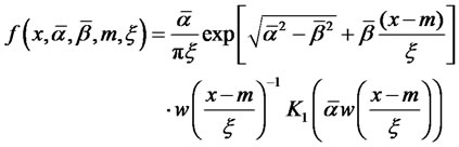 (1)
(1)
where  represent the location scale parameters and
  and K1 is the modified Bessel function of index one in third order.
This paper has adopted their NIG-Jump model to develop the conditional EVT with a jump model. One of the major features of the model is that the previous innovations that are modeled as a serially correlated conditional Poisson process feed back into the expected volatility through the GARCH component of conditional variance. This allows for conditional contemporaneous leverage effects and lagged leverage effects, as described by Maheu and Mccurdy [23].
The market return is expressed as
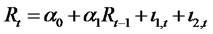 (2)
(2)
where  is the conditional mean and
  is the return innovation at time t, expressed as
 (3)
(3)
while  is a jump innovation with a conditionally mean zero and is contemporaneously independent of
 .
.
The conditional jump intensity λt is expressed as
 (4)
(4)
This parameterization incorporates an autoregressive conditional intensity governing the likelihood of the arrival of jumps between t – 1 and t. δt – 1 is a time-varying intensity residual. It is defined as
 (5)
(5)
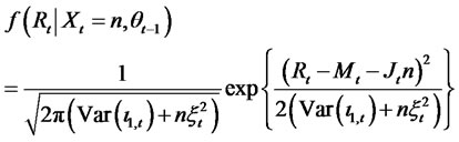
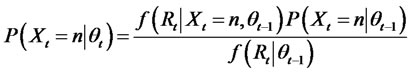
The jump dynamic is assumed to follow a Poisson distribution. The conditional density of Xt is expressed as
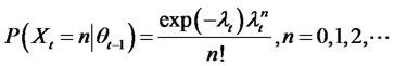 (6)
(6)
where 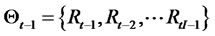 represents the information of the previous return.
The jump size Jt,n follows a normal distribution with mean J and variance ξ.
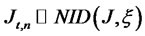 (7)
(7)
Hence, the jump innovation is expressed as
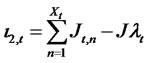 (8)
(8)
This is the sum of Xt jumps arriving within the time interval between  and t and is conditionally mean zero.
The conditional volatility of market returns is governed by two conditional variances as follows:
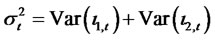 (9)
(9)
The first component describes the diffusion of past information impacts and is defined as a GARCH model:
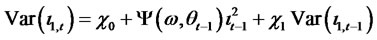 (10)
(10)
where ιt−1 is the total innovation of return at  and is defined as
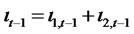 (11)
(11)
Ψ(.) is expressed as
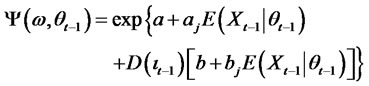 (12)
(12)
where  is the vector of parameters.
  is 1 when
  and 0 otherwise.
  is the expected number of jumps in the time interval between
  and
and . The conditional variance
  is related to the heterogeneous information arrival process that generates jumps, and is expressed as
 (13)
(13)
where Jt is the conditional jump size at time t and is expressed as a function of the past return.
 (14)
(14)
and
 (15)
(15)
where 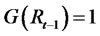 if
if  and 0 otherwise.
The parameters are estimated using the maximum likelihood method. The density function of the return conditional on the most recent information is expressed as
 (16)
(16)
Integrating over the number of jumps, the conditional density function is
 (17)
(17)
The filter is defined as
 (18)
(18)
 .
.
Instead of solving the infinite summation, this paper truncates the summation at 25 for estimating the parameters.
2.1.2. Conditional EVT-NIG + Jump Model
This study incorporates the NIG + Jump model with the EVT to model the time-varying return distribution. This approach focuses on the entire distribution rather than the tail distribution only [14,23] and estimates VaR via a two-stage process. The procedure starts with the NIG + Jump model to estimate the conditional mean and volatileity of the entire distribution. Then, in the second stage, the POT method of EVT is used to model the distribution of the residual.
The parameter vector Q of the NIG + Jump model can be estimated by maximizing the log likelihood function discussed in (16) for N observations.
 (19)
(19)
For the parameter estimation, N is fixed as 1000 (a window of 1000 trading days) and y as 100. With the set of parameters Q, the series of N conditional means and standard deviations can be established.
Then, in stage 2, the series of N residual gt values is calculated based on the formula,
 (20)
(20)
where Mt and σt represents the conditional mean and standard deviation.
Assume Rt follows a distribution Fx. Then, based on the approach of exceedances over thresholds [24-26], by fixing a high threshold τ, the excess distribution of residual gt is expressed as
 (21)
(21)
where , and R0 represents the right endpoints of F [14].
Balkema and de Haan [27] and Pickands [28] stated that Ft(y) tends to a GPD for a large class of distribution F, expressed as
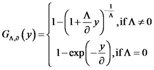 (22)
(22)
where y = Ri-t and Λ represents the tail index, while ¶ is the scaling parameter.
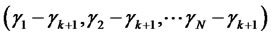
The threshold value affects the distribution of extreme values. Bali [9] set the threshold as twice the standard deviation around the sample mean of the asset value. This study, however, followed McNeil and Frey’s [16] method for determining the threshold. For every N (number of daily observations), let k be the number of points that exceed the threshold. I can then develop a random threshold  at the (k + 1)th order statistic. By ordering the residuals as
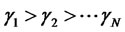 , the GPD distribution can then be fitted to the data series of excess amount of residual over threshold
 . If the threshold is large enough to reduce the chance of bias and k is IID and follow a GPD distribution, the parameters Λ and ¶ can be estimated by the maximum likelihood method [26]. The log likelihood function is expressed as
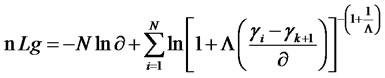 (23)
(23)
The tail estimator is thus given as
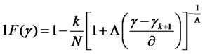 (24)
(24)
I follow the method of McNeil and Frey [16] to take N = 1000 and k = 100 and rank the residuals in ascending order. The residual  is taken as a random threshold to estimate the excess amount of the threshold over the first 100 residuals
 . The VaR estimate using the conditional EVT via the NIG + Jump model can then be computed as
 (25)
(25)
2.2. VaR Estimates Using the Student-t Distribution and the GARCH Model
This study followed Lin and Shen’s [29] model for estimating VaR using the Student-t distribution along with a GARCH model. The density function of a non-central Student-t distribution is denoted as
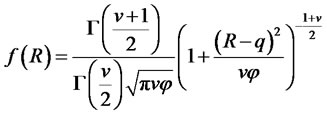 (26)
(26)
where q and j are the location and dispersion parameters, respectively. n denotes the degrees of freedom, and G(·) is the gamma function.
At p percent of the Student-t distribution, the VaR estimate is expressed as
 (27)
(27)
where tp,n represents the corresponding critical t-value and k is the excess kurtosis.
The daily VaR quantiles via the GARCH and NIG + Jump models are then determined by incorporating the corresponding variance into Equation (29). The process was repeated on a rolling basis for the entire set of data.
3. Empirical Analysis
3.1. Data
Three stock indices, the Dow Jones Industrial Average Index (Dow Jones), the Bombay Stock Exchange Sensitive Index (Sensex) and the Thailand Stock Exchange Index (SET), were selected to test the models’ performance. Daily observations range from January 1, 1985 to May 19, 2009. To examine the performance of the VaR models in financial crisis events like the Asian financial crisis, this paper used SET data from Thailand for examination.
Table 1 summarizes the statistics for the daily returns of the three indices. It shows that Sensex has the highest standard deviation (1.85 percent) while Dow Jones S&P has the lowest (1.11 percent). The Dow Jones index represents a developed country while Sensex and SET represent the emerging markets of Asia. Therefore, they generally exhibit higher volatility. In addition, the distributions of the three return series are heavily tailed. The kurtosis and skewness are relatively higher for the Dow Jones. The Jarque-Bera statistics for the three indices are exceptionally high, which evidences the non-normality of these distributions.
3.2. Parameter Estimation
The parameter estimates of the models are determined by the maximum likelihood method, with the results presented in Tables 2 and 3. A window of 1000 daily observations is used to estimate the parameters for next-day estimation. The results show that the tail indices Λ for the EVT-based models are positive. Therefore, the limiting distributions of the three indices are of the Fréchet type.
3.3. Empirical Tests
Three sets of tests were conducted to measure each model’s performance related to in-sample fitting, out-ofsample forecasting and backtesting by years.
In-sample testing measures how good each model is at fitting the data. The out-of-sample study, acting as a
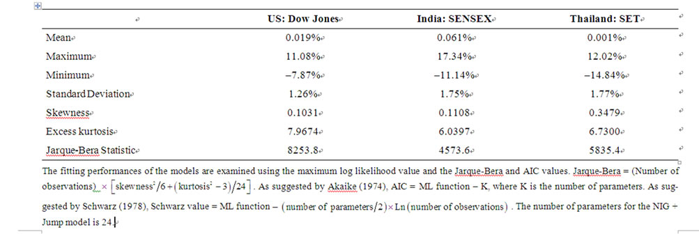
Table 1. Summary statistics of the stock index returns. Panel A (Parameters—Part: NIG + Jump).
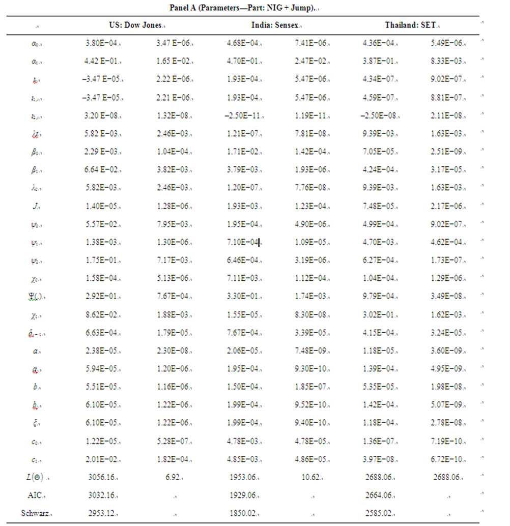
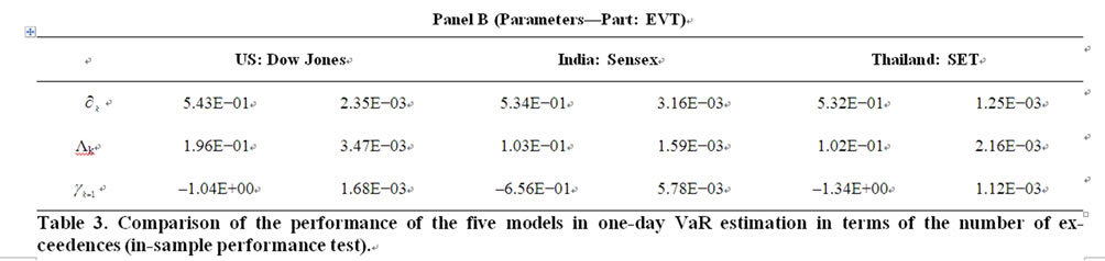
Table 2. Estimation of parameters of the EVT-NIG + Jump model for the stock index returns.
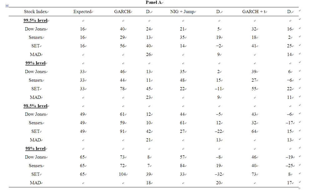
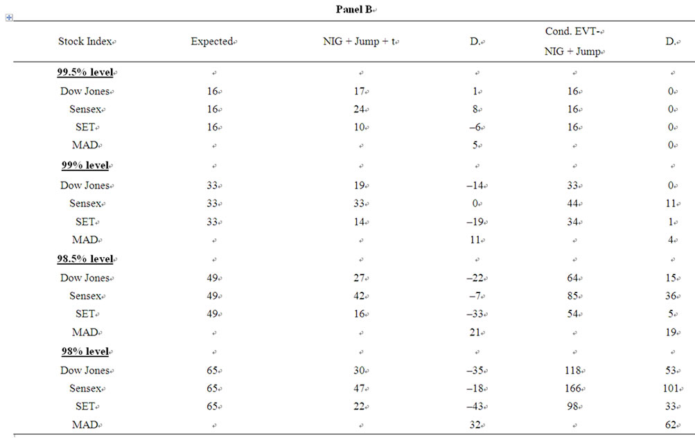
Table 3. Comparison of the performance of the five models in one-day VaR estimation in terms of the number of exceedences (in-sample performance test).
back-test, compares the actual return with the daily VaR forecasts throughout the sample period to evaluate each model’s performance in forecasting VaR estimates. The backtest is analyzed on an annual basis to examine each model’s ability to capture the dynamics of conditional volatility of the indices. The five models for comparison are the GARCH, NIG + Jump, GARCH-t, NIG + Jump-t and EVT-NIG + Jump models.
3.3.1. In-Sample Performance
Each model’s parameters were estimated by the maximum likelihood method using the in-sample data. The VaR quantiles for the corresponding confidence level for each date are calculated, and VaR forecasts of the five models are then compared against the actual daily return for each index.
Table 3 indicates the relative in-sample performance of the five models in one-day VaR estimation. Since the best model for VaR measurement should give the exact number of expected exceedences, the EVT-NIG + Jump model outperforms the other five models by giving the smallest deviation of its number of exceedences from the expected figures at both the 99 percent (one percent of the number of daily observations in the sample period) and 99.5 percent level for all three stock indices. The EVT-NIG + Jump model is better than the conditional EVT model for both the Dow Jones index and the two indices of emerging markets. It seems that the jump process is better at capturing event losses due to unusual events. The autoregressive conditional intensity governing the jump process allows the news feedback on variance from jumps to vary when the previous news is good or bad. This helps the jump-based models to better capture the non-normality when estimating VaR. It is shown that the NIG + Jump-based models, such as the NIG + Jump-t model, are better than GARCH without the jump model in VaR forecasting. The performances for the conditional EVT-based models are generally better than those of the GARCH-based models. The EVT-NIG + Jump model has the lowest MAD among the five models.
Comparing the GARCH type models, it is found that the NIG + Jump-t model yields the best prediction of VaR for all three indices. While exhibiting a higher MAD in a lower confidence level, its prediction improves substantially at higher confidence levels. It has the lowest MAD among the GARCH type models at both the 99 and 99.5 percent level. At the 99.5 percent level, the ranking of performance starting from the best is EVT-NIG + Jump, NIG + Jump-t, GARCH-t, NIG + Jump, and GARCH. At the 99 percent level, the EVT-NIG + Jump model still outperforms the other models in providing the lowest absolute deviation from the expected figures. The MAD is only four. The NIG + Jump-t model outperforms the other GARCH type models.
From the 98.5 percent to 95 percent level, the EVTNIG + Jump model still ranks the best. It gives the lowest number of absolute deviations from the expected figures. The performance of the NIG + Jump model, however, improves at lower confidence levels. It has the lowest MAD in the 98.5 to 97.5 percent level, as compared with the other GARCH type models. It seems that the combination of NIG + Jump and the t distribution leads to an over-prediction of VaR and generates a higher MAD. It is inferred that the performance of the EVT-NIG + Jump model improves as the confidence level increases. The conditional EVT series models generally perform better with the Dow Jones Index than with the Sensex and SET, especially at higher confidence levels, due to the larger volatility clustering and kurtosis that exists in the Dow Jones. The EVT-NIG + Jump model does a good job in capturing these non-normalities.
3.3.2. Backtesting (Out-of-Sample) Performance
The five models were backtested to examine how well the models predict extreme losses in the future. This is particularly important for short-term market risk management, by evaluating each model’s performance in VaR forecasting. Backtesting starts with a window of 1000 previous daily observations in the sample to estimate the parameters of each model. The estimates are then used to derive the one-day VaR forecast for the next day, and the forecasts are compared with the actual return of that day. The procedure is repeated for the rest of the daily observations in the sample. The exceedences are counted whenever the actual return is lower than the VaR forecasts. The results are summarized in Table 4.
Compared with the results in Table 3, Table 4 generally has higher numbers of exceedences for all models in the out-of-sample test. At the 99.5 percent level, the order of ranking in terms of the number of exceedences remains the same as that in Table 3. EVT-NIG + Jump is still the best model in VaR estimation. In addition, the NIG + Jump-t model outperforms all of the other GARCH type models.
At the 99 percent level, the EVT-NIG + Jump model still produces the fewest outliers in the backtesting. From the 98.5 percent to 95 percent level, the EVT-NIG + Jump model remains the best performer. The ranking is the same as that in the in-sample test, although the number of outliners increases with decreasing confidence levels. In addition, it is shown that the MAD for both the NIG + Jump-t and GARCH-t models increases with decreasing confidence level. This may attribute to the poorer performance of the Student-t function in fitting the actual financial time series distribution as the confidence level decreases. The NIG + Jump model can better forecast unusual news events or earnings surprises with
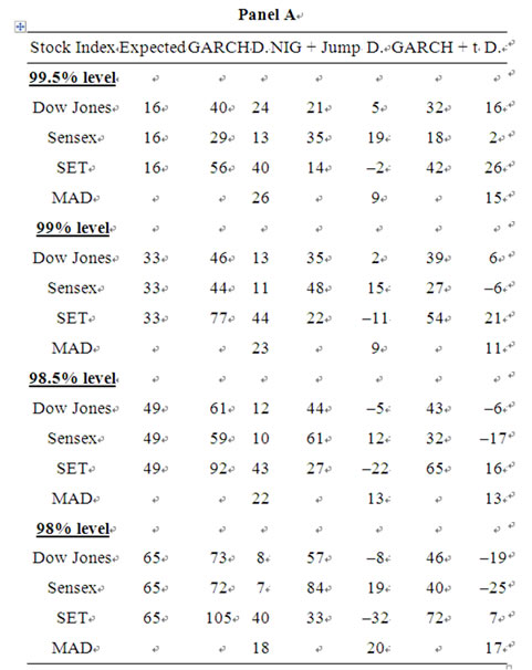
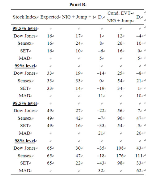
Table 4. Comparison of the performance of the five models in one-day VaR forecasts in terms of the number of exceedences (out-of-sample performance test).
the inclusion of a jump process. The GARCH model, however, which has linear volatility settings, is less sensitive to changes in return volatility [30].
3.3.3. Unconditional and Conditional Coverage Tests
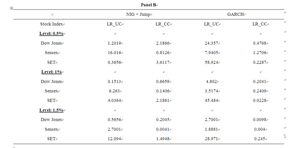
The unconditional coverage test and conditional coverage test were conducted. The unconditional coverage test measures the performance of the VaR models based on the proportion of failures in the sample, while the conditional coverage test tests both the unconditional coverage and serial independence. The derivations of both the unconditional and conditional coverage tests are given in the Appendix.
Table 5. Unconditional coverage and conditional coverage tests for alternative VaR models. Table 5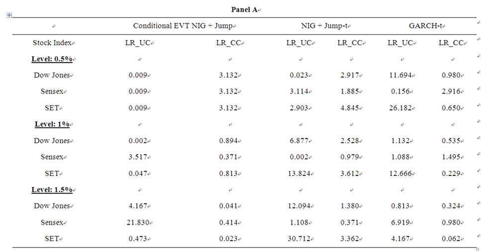
3.3.4. Yearly Backtesting
Byström’s [14] method s adopted to compare the performance of conditional and unconditional models by dividing the sample period into year-long sub-periods. Table 6 presents the comparative performance of VaR forecasts of the five models on an annual basis at the 99 and 99.5 percent levels.
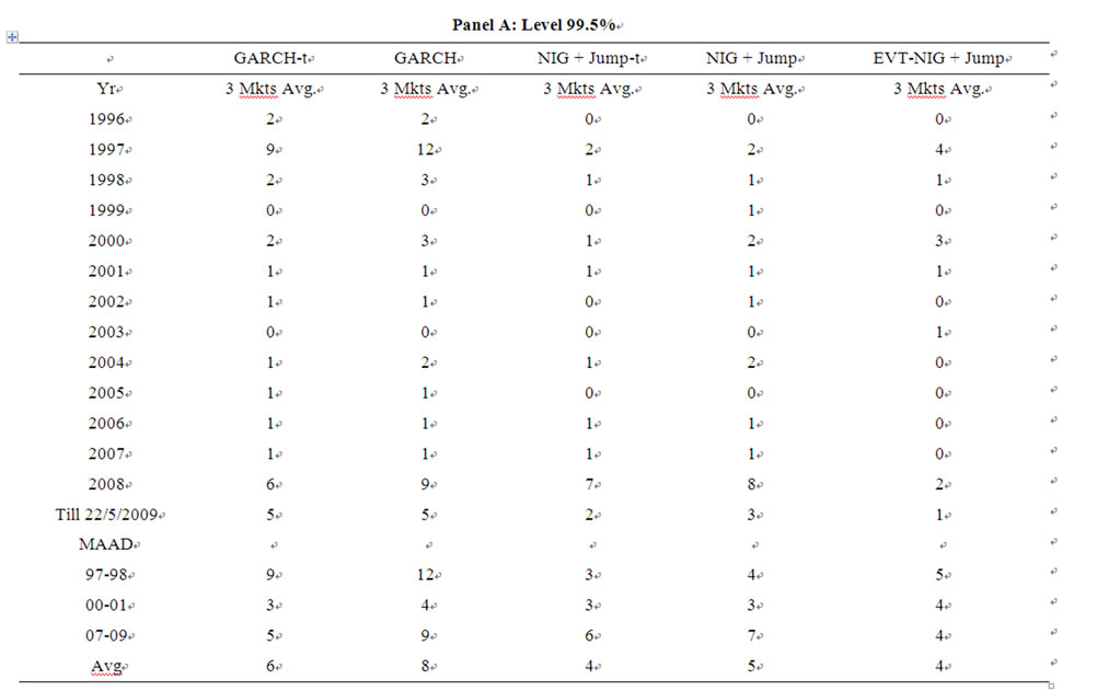
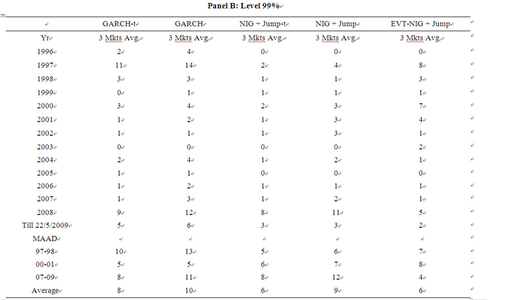
Table 6. Annual backtesting performance in one-day VaR forecasts of the five models at 99.5% and 99% levels (outof-sample test).
The results show that both the NIG-Jump-t and EVTNIG-Jump models generally give a lower MAAD (Mean Average Absolute Deviation). The EVT-NIG + Jump model generates accurate VaR estimates, as expected by the confidence level. The same situation applies to the three stock indices at the 99 and 99.5 percent levels. The daily VaR estimates produced by the conditional EVT models vary closely with changes in volatility. In particular, the EVT-NIG + Jump model captures the extreme losses during the period well for both the Sensex and SET indices.
The VaR forecasts by the GARCH model, however, are less responsive to changing volatility. The GARCH model tends to underestimate the risk during turbulent periods.
In accessing the performance of the VaR forecasts of the five models in the three crises, this paper measures the MAAD of the models for the periods of 1997-1998,2000-2001 and 2007-2009. These periods include the devaluation of stock market values in Asian markets in 1997, the technical bubble burst in 2000 and the collapse of investment banks in 2007. It is shown that both the NIG-Jump-t and EVT-NIG + Jump model perform significantly well in capturing extreme losses. In particular, the EVT-NIG + Jump model gives the lowest average MAAD in the Global Financial Crisis at 99 percent level. It is inferred that the EVT model incorporated with the jump process is more responsive to sudden jumps in stock price and is better at capturing extreme price movements during a crash period.
4. Conclusions
This paper proposes a conditional EVT-based model that incorporates the NIG + Jump process for VaR estimation. It explores the possibility of improving the EVT-based model in estimating and forecasting VaR for extremeevents. The EVT-NIG + Jump model includes an autoregressive jump component in valuing the conditional variance to feedback previous jump innovations into the expected volatility. This feature helps the model perform better around crisis periods.
The findings indicate that the EVT-NIG + Jump model performs well—especially at high confidence levels—in both the in-sample and out-of-sample tests. In the insample test, the EVT-NIG + Jump model outperforms all of the alternative models in scapturing the heavy tail and skewness of the return distribution of the three indices studied. The results show that the VaR model developed in the EVT-NIG + Jump framework is more robust in tracking the occurrences of extreme losses in emerging stock markets, such as those in India and Thailand.
In the out-of-sample test, the EVT-NIG + Jump model again performs well for one-day VaR forecasts. The improvement became more significant when a higher confidence level VaR forecast (99 percent or above) was used. The NIG + Jump setting incorporated in the proposed model helps to better capture the skewness and heavy tail resulting from an unexpected extreme price jump. Additionally, the performance of the conditional NIG + Jump model in VaR forecasts improves as the confidence level increases. The model produces exceptionally accurate VaR forecasting at the 99.5 percent level.
Regarding the year-by-year backtesting, the conditional EVT-NIG + Jump model performs well and outperforms the others in capturing the dynamics of the market condition.
REFERENCES
- P. Artzner, F. Delbaen, J. Eber and D. Heath, “Thinking Coherently,” Risk, Vol. 10, No. 11, 1997, pp. 68-71.
- P. Artzner, F. Delbaen, J. Eber and D. Heath, “Coherent Measures of Risk,” Mathematical Finance, Vol. 9, No. 3, 1999, pp. 203-228. doi:10.1111/1467-9965.00068
- T. G. Bali and P. Theodossiou, “A Conditional-SGT-VaR Approach with Alternative GARCH Models,” Annals of Operations Research, Forthcoming, Vol. 151, No. 1, 2005, pp. 241-267.
- F. M. Longin, “Optimal Margins Level in Future Markets: A Parametric Extreme-Based Method,” Journal of Futures Markets, Vol. 19, No. 2, 1999, pp. 127-152.
- S. C. Coles, “An Introduction to Statistical Modeling of Extreme Values,” Springer, London, New York, 2001.
- F. M. Longin, “From Value at Risk to Stress Testing: The Extreme Value Approach,” Journal of Banking & Finance, Vol. 24, No. 7, 24, 2000, pp. 1097-1130. doi:10.1016/S0378-4266(99)00077-1
- J. Cotter, “Downside Risk for European Equity Markets,” Applied Financial Economics, Vol. 14, No. 10, 2004, pp. 707-716. doi:10.1080/0960310042000243547
- T. G. Bali, “A Generalized Extreme Value Approach to Financial Risk Measurement,” Journal of Money, Credit and Banking, Vol. 39, No. 7, 2006, pp. 1613-1649.
- T. G. Bali, “An Extreme Value Approach to Estimating Volatility and Value-at-Risk,” Journal of Business, Vol. 76, No. 1, 2003, pp. 83-108. doi:10.1086/344669
- T. G. Bali and S. N. Neftci, “Disturbing Extremal Behavior of Spot Rate Dynamics,” Journal of Empirical Finance, Vol. 10, No. 4, 2003, pp. 455-477. doi:10.1016/S0927-5398(02)00070-1
- J. Beirlant, J. Teugels and P. Vynckier, “Practical Analysis of Extreme Values,” Leuven University Press, Leuven, 1996.
- P. Embrechts, C. Klüppelberg and T. Mikosch, “Modelling Extremal Events for Insurance and Finance,” SpringerVeriag, New York, 1997.
- R. Reiss and M. Thomas, “Statistical Analysis of Extreme Values: From Insurance, Finance, Hydrology, and Other Fields,” Birkhäuser Verlag, Basel, Boston, 2001.
- H. N. E. Byström, “Managing Extreme Risks in Tranquil and Volatile Markets Using Conditional Extreme Value Theory,” International Review of Financial Analysis, Vol. 13, No. 2, 2004, pp. 133-152. doi:10.1016/j.irfa.2004.02.003
- R. Smith, “Measuring Risk with Extreme Value Theory,” Extremes and Integrated Risk Management, Vol. 2, 1996, pp. 19-36.
- A. J. McNeil and R. Frey, “Estimation of Tail-Related Risk Measures for Heteroscedastic Financial Time Series: An Extreme Value Approach,” Journal of Empirical Finance, Vol. 7, No. 3-4, 2000, pp. 271-300. doi:10.1016/S0927-5398(00)00012-8
- T. G. Bali and D. Weinbaum, “A Conditional Extreme Value Volatility Estimator Based on High-Frequency Returns,” Journal of Economic Dynamics and Control, Vol. 31, No. 2, 2007, pp. 361-397.
- C. Brooks, A. D. Clare, J. W. D. Molle and G. Persand, “A Comparison of Extreme Value Theory Approaches for Determining Value at Risk,” Journal of Empirical Finance, Vol. 12, No. 2, 2005, pp. 339-352. doi:10.1016/j.jempfin.2004.01.004
- R. F. Engle, “Autoregressive Conditional Heteroscedasticity with Estimates of the Variance of UK,” Econometrica, Vol. 50, No. 4, 1982, pp. 987-1008. doi:10.2307/1912773
- T. P. Bollerslev, “Generalized Autoregressive Conditional Heteroscedasticity,” Journal of Econometrics, Vol. 31, No. 3, 1986, pp. 309-328. doi:10.1016/0304-4076(86)90063-1
- S. Taylor, “Modelling Financial Time Series,” In: H. Akaike, Ed., A New Look at the Statistical Model Identification, John Wiley & Sons, New York, 1986.
- R. Susmel, “Switching Volatility in Private International Equity Markets,” International Journal of Finance & Economics, Vol. 5, No. 4, 2000, pp. 265-283. doi:10.1002/1099-1158(200010)5:4<265::AID-IJFE132>3.0.CO;2-H
- J. M. Mahe, and T. H. McCurdy, “News Arrival, Jump Dynamics, and Volatility Components for Individual Stock Returns,” Journal of Finance, Vol. 59, No. 2, 2004, pp. 755-793. doi:10.1111/j.1540-6261.2004.00648.x
- A. C. Davison and R. L. Smith, “Models for Exceedences over High Thresholds,” Journal of the Royal Statistical Society, Vol. B52, No. 3, 1990, pp. 393-442.
- M. R. Leadbetter, “On a Basis for Peaks over Thresholds Modeling,” Statistics and Probability Letters, Vol. 12, No. 4, 1991, pp. 357-362.
- R. Smith, “Extreme Value Analysis of Environmental Time Series: An Application to Trend Detection in GroundLevel Ozone,” Statistical Science, Vol. 4, No. 4, 1989, pp. 367-393. doi:10.1214/ss/1177012400
- A. Balkema and L. de Haan, “Residual Life Time at Great Age,” Annals of Probability, Vol. 2, No. 5, 1974, pp. 792- 804. doi:10.1214/aop/1176996548
- J. Pickands, “Statistical Inference Using Extreme Order Statistics,” The Annals of Statistics, Vol. 3, No. 1, 1975, pp. 119-131. doi:10.1214/aos/1176343003
- C. H. Lin and S. S. Shen, “Can the Student-t Distribution Provide Accurate Value at Risk?” The Journal of Risk Finance, Vol. 7, No. 3, 2006, pp. 292-300. doi:10.1108/15265940610664960
- M. Y. L. Li and H. W. W. Lin, “Estimating Value-at-Risk via Markov Switching ARCH Models: An Empirical Study on Stock Index Returns,” Applied Economics Letters, Vol. 11, 2004, pp. 679-691.
Appendix: Unconditional Coverage and Conditional Coverage Test
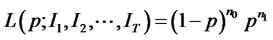
The likelihood ratio test for unconditional coverage is
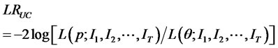 (A1)
(A1)
where q = n1/(n0 + n1) and ni is the number of observation with value I and
The likelihood ratio test for conditional coverage is
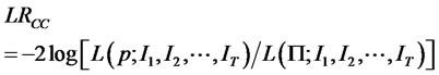 (A2)
(A2)
where
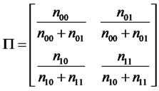
nij is the number of observations with value i followed by j.