Open Journal of Marine Science
Vol.05 No.02(2015), Article ID:55174,16 pages
10.4236/ojms.2015.52016
Characteristics of Tides in the Red Sea Region, a Numerical Model Study
Fawaz Madah, Roberto Mayerle, Gerd Bruss, Joaquim Bento
Coastal Research Laboratory-CORELAB, Research and Technology Centre West Coast (FTZ), University of Kiel, Kiel, Germany
Email: fmadah@corelab.uni-kiel.de
Copyright © 2015 by authors and Scientific Research Publishing Inc.
This work is licensed under the Creative Commons Attribution International License (CC BY).
http://creativecommons.org/licenses/by/4.0/


Received 26 January 2015; accepted 26 March 2015; published 30 March 2015
ABSTRACT
In this work, a two-dimensional numerical model based on Delft3D modelling system was setup to study the tidal characteristics of the Red Sea. Besides that, analyses of available observed time series of surface elevations were carried out. Sensitivity analyses of the numerical model were carried out by testing different model parameters aiming at selecting optimal settings. The model performance was evaluated against available time series of surface elevation observations. RMS error was found to vary from 0.03 to 0.1 meter, while the ADM values range from 0.02 to 0.05 meter. On the whole, the model is able to reproduce the tidal wave in the Red Sea, reflecting a consistent level of agreement with the observations and previous works. The model results suggest that the semidiurnal tidal waves play a major role in the region except in the central part of the Red Sea where amphidromic system exists. Major semidiurnal and diurnal tidal constituents were computed to generate co-charts and form factor. The results have revealed that the distribution of the co-charts of the major semidiurnal constituents M2, N2, and S2 show the existence of anticlockwise amphidromic system in the central part of the Red Sea at about 19.5˚N, north of the Strait of Bab el Mandeb at 13.5˚N and in the Gulf of Suez. The chart of the diurnal tidal constituent K1 showed a single counterclockwise system in the southern part of the Red Sea centred around 15.5˚N. The form factor chart shows the appearance of diurnal character in the central part of the basin and the northern end of the strait. The hydrodynamics patterns under spring and neap tidal conditions were also analysed (during flood and ebb conditions). Model results showed that currents generally are weak and strongest currents are present in the strait of Bab el Mandeb and Gulf of Suez.
Keywords:
Red Sea, Delft3D Modelling System, Amphidromic System, Co-Charts

1. Introduction
Tides are the periodic motion in sea level resulting from the gravitational force of the moon and the sun and the centrifugal force generated as the earth rotates about the common centre of mass earth-moon-sun system. A basic knowledge of ocean dynamic particularly tides propagation at any place is a prerequisite to predict problems such as pollution, dispersion, sediment transport, etc. on coastal regions. Tidal currents influence the erosion processes occurring daily, and hence affect the nutrients budgets [1] [2] . The Red Sea is an elongated-shaped basin (semi-enclosed), extending from NNW to SSE (30˚N to 12˚N latitude and 32˚E to 44˚E longitude) over a distance of about 2000 km and separates the African and Asian landmass (Figure 1). The physical boundary of the Red Sea is delineated by the coastline of Egypt, Sudan, Eritrea and part of Djibouti in the western side and the coastline of Jordan, Saudi Arabia and Yemen on the eastern side. In the southern part of the basin, it links with the Gulf of Aden and the Indian Ocean through a narrow, shallow strait (26 km wide, 150 km long) known as Bab el Mandeb while in the north it consists of the so-called Gulf of Suez and Gulf of Aqaba [3] -[6] . The Red Sea experiences irregular bottom topography. The average depth is about 490 m while maximum depth > 2000 is found in the axial trough. The Red sea has a surface area of about 450,000 km2. In the southern part of the basin, there are shallow shelves on both sides of the strait of Bab el Mandeb linking the Red Sea with the Gulf of Aden, the shallowest Sill known as Hanish Sill is located at the northern part of the Strait and the narrowest contraction is located at the Perim Narrows in the southern end of the strait [7] . The Red Sea contains a unique large marine ecosystem. Most of the coastline of the Red Sea is bordered by a coral reef system, thus tide and
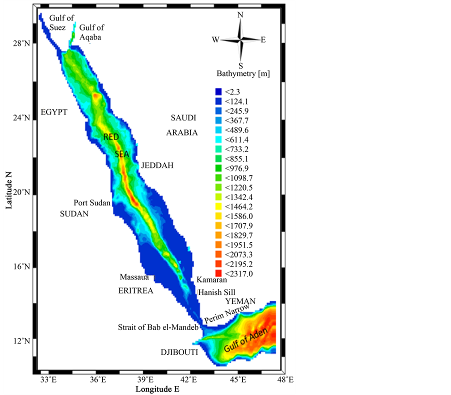
Figure 1. Geographic location of the Red Sea and the numerical bathymetry based from the global bathymetry datasets for the world ocean “GEBCO_08”.
associated currents basically are important components for ecological and relevant environmental studies. On the other hand, the Red Sea is an important international shipping path linking eastern and southern Asia with the Middle East and Europe. Despite its socio-economic and environmental importance, there is very little published information regarding tidal characteristics in the region. The earlier works on tides were basically limited to observations which are confined to the coastal region [6] [8] [9] . During the last century, a dynamical explanation of actual tides was supplied based on theoretical study. Studies on tides based on numerical modelling approach do not exist. Many researchers emphasize the necessity of numerical modelling approach to advance basic understanding of the region where there is lack of understanding the physical system regulating the marginal seas and Gulfs in the region [10] . Consequently, it is of interest to carry out a study of tides in the Red Sea using a modelling approach. Therefore, this research focuses on tidal characteristics in the Red Sea region by means of implementation and application of a numerical modelling method and by analysing its results. The specific model used to achieve this study is Delft3D modelling system, developed by Delft Hydraulics in the Netherlands. Besides that, available observations of surface elevations in the region were also considered in this study.
This paper is organized as follows. In section 1.1, a review of the study area is presented. In section 1.2, the available observations of surface elevation are analyzed. Section 2 introduces a brief description of the modelling system used in this investigation, followed by the setup of the Red Sea model (RS-Model) including processes involved in the setup and model performance. Section 3 presents the results of the numerical simulations including the tidal characteristics based on the distributions of co-range and co-tidal charts, form factor and hydrodynamic features. Section 4 throws light on the conclusion of this study.
1.1. General Review
A general description regarding the physical characteristics of the Red Sea such as wind conditions, water temperature, salinity, heat flux, etc, is found in the previous studies of [5] [11] -[19] . Generally, the climate of the Red Sea region is a typical desert and semi-desert climate characterized by high temperatures, low rainfall with an average of 109 mm/year. The northern part of the Red Sea is under the influences of the eastern Mediterranean weather system. South of 18˚ latitude including the Gulf of Aden region is mainly controlled by the Indian monsoon system, north-easterly monsoon (October to May) and a south-westerly monsoon (June to September). The evaporation rate in the Red Sea is very high compared to other oceans and seas. Fresh water is negligible due to low precipitation and absence of river discharge. As a result, highly saline conditions are found in the Red Sea (42 psu).
Very little information is found concerning tides in the literature. The tides in the Red Sea have been described by [20] based on a few analytical analyses carried out in order to determine the tides in the strait of Bab el Mandeb and the results of these analyses were used to explain tidal dynamics in the whole Red Sea basin. The conclusion drawn suggests that the tidal regime in the Red Sea is essentially co-oscillations with those of the Gulf of Aden, characterized by its low tidal range with semidiurnal characteristics. There is a difference of six hours between the time of high water in the north and in the south. This means that high water at the southern end of the Red Sea signals low water at the northern part and vice versa. The tidal range changes from north to south with greatest values at the two ends. In the north, at the entrance of Suez and Aqaba Gulfs the spring range is about 0.6 m while in the southern part of the Red Sea (at Massawa and Kamaran Island) is around 0.9 m. However, the range decreases towards the central part of the Red Sea near Jeddah and Port Sudan where amphidromic system (counter-clockwise) exists due to the M2 tidal wave. There are also another two nodal zones that exist across the Red Sea with negligible tide occurring to the north of Bab el Mandeb and at the entrance of the Gulf of Suez. Generally, in places where the semidiurnal tides are very weak, diurnal character may appear. Nevertheless, it has been pointed out by [12] that there is disagreement on a complete explanation of the Red Sea tides.
Reference [9] analyzed time series of hourly sea level records for one year at two stations located in the central part of the Red Sea (Jeddah and Port Sudan). Their analysis showed that the tide at Jeddah can be classified as mixed type dominated by semidiurnal tide. On the other hand, their results indicated that the semidiurnal components (M2, S2) at Port Sudan are smaller in comparison with those at Jeddah and the amplitudes of the fortnightly and monthly components are larger. Based on the form ratio (F) value, the tide at Port Sudan was found to be of diurnal type. This was explained on the basis of the proximity of Port Sudan to the amphidromic point. Reference [6] performed harmonic analysis of hourly sea level records for the period (1992-1994) in the southern part of the Red Sea at JIZAN (Lat 16˚53'N, Long 42˚35'E). His analysis showed that the tide at JIZAN is dominated by the large amplitudes of the major semidiurnal constituents M2, S2, and N2. Diurnal components on the other hand (O1, K1) were the smallest amplitudes among the others. Using the form ratio (F) to determine the character of the tide, it was found that the ratio was less than 0.25 indicating the type of semidiurnal tide.
Observational studies on water currents inside the Red Sea domain are very limited, and the patterns that emerged from the observations are significant northward currents close to the western coast in the southern part of the Red Sea during winter [21] and southward counter-current at depths greater than 250 m in the central part of the Red Sea in the open sea but less than 150 m near the coast of Port Sudan [22] ; a cyclonic gyre at the extreme north (north of 23˚ latitude) which penetrates up to 300 m depth and an anticyclonic gyre about 2˚ to the south [4] [14] [19] [22] [23] . These previous studies are basically attributing and discussing the importance of the wind effects and thermohaline forcing on the generated currents. In the past century, the area that attracted the researchers is the strait of Bab el Mandeb. As a result, most of the observational studies were carried out in the vicinity of Bab el Mandeb strait which were aimed at understanding the exchange between the surrounding water bodies. The results of these investigations suggest that there is a 2-layer exchange flow system in a winter period from October to May, with surface inflow and a deep outflow characterized by very saline (40 psu) Red Sea Outflow Water (RSOW). In a summer season (June-September) the system of 2-layer is replaced by a 3- layer flow system; shallow surface outflow, subsurface intrusion of Gulf of Aden Intermediate Water (GAIW) and a deep RSOW [7] [13] [24] -[26] .
1.2. Tidal Characteristics Based on Observations
This section presents the tidal characteristics in the Red Sea based on the tidal constituents produced from the harmonic analysis of the available tidal observations. During this research the available data are the tidal elevations in the region of the Red Sea from five tide gauges stations along the eastern coast of the Red Sea (JIZAN, JEDDAH, YANBU, RABIGH and DUBA) operated by Saudi ARAMCO Oil Company, three new tide gauges were installed in 2011 in the vicinity of JEDDAH coastal waters at the Coast Guard Stations of Obhor Creek, Gahaz and Saroom via the Faculty of Marine Sciences (King Abdulaziz University, Saudi Arabia) and Research and Technology Centre-CORELAB (University of Kiel, Germany) and data from one location on the western coast at Port SUDAN. In addition to that, time series of water level records from two additional stations located in the Gulf of Aden (at Aden and Djibouti) obtained from the Sea Level Centre at University of Hawaii (UHSLC) were made available (see Figure 3 for their locations). The purpose of using these data on the one hand is to perform tidal analysis and determine the major semidiurnal and diurnal constituents and on the other hand to be used for calibration and validation of the RS-Model. The length of the time series was one year at hourly intervals. Tidal analyses were performed using the World Tides program ver. 2009 [27] to compute the amplitudes and phases of the eight primary semidiurnal and diurnal tidal constituents (Q1, O1, P1, K1, N2, M2, S2 and K2). Examples of tidal amplitudes obtained from this analysis at some stations (ADEN, JIZAN, JEDDAH, RABIGH, DUBA and SUDAN) are shown in Figures 2(a)-(f). The figures obviously display a change in the tidal regime and range. It is clear that the tides of the Red Sea are relatively small and the magnitude varies according to the location. On the other hand, the magnitude of the tidal amplitude at Aden (Figure 2(a)) behaves differently, indicating different tidal regime characterized by a mixed type with diurnal and semidiurnal fluctuations. The figure shows that the major semidiurnal constituents are M2 (principal lunar with a period of 12.42 hours), S2 (principal solar with a period of 12.00 hours) and N2 (larger elliptic lunar with a period of 12.66 hours) respectively, while the major diurnal tide is K1 (principal luni-solar with a period of 23.93 hours). It is clear that the amplitudes of semidiurnal tidal constituents at SUDAN (Figure 2(f)) are smaller than diurnal constituents. Inside the Red Sea domain, the contribution of the semidiurnal constituents M2, S2 and N2 for the total astronomical tide represents larger portion at location B, D and E. This indicates that the total astronomical tide is well represented by the major tidal constituents. On the other hand, the contribution of most other constituents on the total astronomical tide suggests that the constituents with smaller amplitude than the K1 may be ignored.
2. Model Setup
Only few observed data were found to be available in the area of interest during this research. Taking into consideration the length of the Red Sea, the availability of tide gauge data only at a few locations may not reflect a complete picture about the tidal characteristics in the region. However, considering the advantages of using a

Figure 2. Amplitudes of semidiurnal and diurnal tidal constituents based on the tidal analysis, (a): ADEN; (b): JIZAN; (c): JEDDAH; (d): RABIGH; (e): DUBA; (f): SUDAN.
numerical modelling approach, the development of a numerical model and its application maybe a good alternative to carry out such study and provide a comprehensive picture about the tidal characteristics in the Red Sea. Two dimensional models, namely the depth-averaged or shallow water models, can be successfully applied for simulating tidal flow and flows of water bodies.
2.1. Model Description
In the present work, the Delft3D modelling system developed by WL|Delft Hydraulics in the Netherlands was used. The system is a fully integrated program which simulates the time and space variations of six phenomena namely hydrodynamics, wave interaction, water quality, morphology, sediment transport and ecology in addition to their interactions. The Delft3D-Flow is (the basic module in the system) a multi-dimensional (2D or 3D) hydrodynamic model which aims to solve non-steady flows and transport phenomena resulting from tidal and meteorological forcing including the effects of density differences (due to temperature and salinity distribution) on a rectilinear or curvilinear boundary fitted grid. It can be used to simulate flows in shallow seas, coastal areas, estuaries, lagoons, river and lakes. The equations of the system are derived from the three dimensional Navier Stokes equations for an incompressible free surface flow, under the shallow water and the Boussinesq assumption [28] . The system of equations consists of the horizontal equations of motion, the continuity equation and the transport equations for conservative constituents. The numerical solution of the equations is obtained by discretizing the equations in space using an explicit finite difference scheme over a uniform staggered Arakawa-C grid [29] and in time using Alternating Differential Implicit (ADI) technique. The ADI method divides one integration time step into two phases; each phase consists of half a time step [2] [30] . Since the solution is implicit, numerical stability is not limited by the time step, however, the accuracy of the flow decreases with increasing time step from accurate solutions when the Courant number is less than  [31] .
2.2. Model Domain and Bathymetry
After gathering the input data needed for setting up the model including the bathymetry of simulation area and boundary condition, Delft-RGFGRID program was utilized to construct the grid. Figure 3 shows the resulting

Figure 3. Computational grid distribution of the Red Sea model (RS-Model), red line represents the open boundary and green colour represents closed boundaries, [Black dots indicate the locations of the tidal gauge stations used in the model calibration and validation].
computational grid of the RS-Model where green colour represents the closed boundary while the open boundary is marked by red colour. The figure also includes the locations of the available surface elevation observations used for calibration and validation processes. The RS-Model domain covers the entire Red Sea and extends to the eastern part of the Gulf of Aden (48˚E). The model domain was schematized on a rectangular mesh with a uniform grid spacing of 5 km horizontally. The total number of elements grid used in the computation consists of 63,434 grid cells. The coordinates system of the grid is spherical and therefore the variation of the Coriolis force is determined in the latitude direction.
The bathymetric data of the RS-Model were sourced from the global bathymetry dataset for the world ocean ‘‘GEBCO_08 Grid’’ at a 30 arc-second horizontal resolution (~1 km) (The GEBCO_08 Grid, version 20090202, http://www.gebco.net/). Data for the RS-Model domain were extracted and converted into the appropriate file format. Figure 1 shows the resulting bathymetric map based from this data. Due to insignificant artificial contact between the Red Sea and the Mediterranean via Suez Canal, the model has only one open boundary which was set at the Gulf of Aden at longitude (48˚E) and divided into 25 segments. Due to unavailability of measurements near the open ocean boundary, tidal amplitudes and phases of the main semidiurnal and diurnal tidal constituents (Q1, O1, P1, K1, N2, M2, S2 and K2) extracted from the global ocean tidal model TPXO 7.2 on 1/4 × 1/4 degree resolution global grid were prescribed at boundary cells and linearly interpolated. A free slip condition was applied on the closed boundaries with a zero value of normal velocity. A time step of 60 seconds was set in all simulations to insure the stability and accuracy of the model. Initial conditions of water levels were set equal to zero in all simulations. As a result, the equilibrium state in terms of water levels is reached after certain time; therefore, the first four days of the simulation were discarded. Values of water density and gravitational acceleration were set 1025 kg∙m−3 and 9.81 ms−2, respectively.
2.3. Tuning the RS-Model
Since the approximation, simplification and the assumptions are applied in the numerical solution, which leads to differences between the model results and the observations, it is necessary to test the model inputs to insure that the model reproduce accurately the processes which were observed in reality [32] . Accordingly, various sensitivity analyses were carried out to analyze the effect of variations of different parameters on the hydrodynamic model results. This includes boundary condition, eddy viscosity, bottom roughness, mesh resolution, and time step. An early test of the numerical simulation was carried out to check the open boundary conditions. It was found that the model produces similar trend of variations of simulated and observed water level, however, discrepancies related to phase lag conditions were observed. Therefore, adjustments to the open boundary conditions were considered. Three different grid resolutions were tested in the purpose of selecting optimal grid spacing. This analysis revealed that the model is sensitive to grid resolution. Once a mesh grid was adopted, several computational scenarios for different time steps were carried out. This analysis revealed that the model is insensitive to time steps. However, a time step of 1 minute was adopted for stability and accuracy of the numerical model. Bottom roughness is one of the most important parameters in the hydrodynamic models. The Che’zy coefficient depends on the bottom roughness and the height of the water column. Sensitivity tests of Che’zy coefficient on the model results were carried out by testing three spatially and temporally uniform roughness values starting from 45, 65 and 85 m1/2/s, respectively. It was found that using lower or higher value from the initial default value (65 m1/2/s) given by Delft3D-Flow system produce insignificant influences on the model results. Therefore, a constant temporal and spatial value of 65 m1/2/s was adopted and applied throughout the model domain. Another important parameter is horizontal eddy viscosity (HEV) due to its role in defining the turbulence mixing in the water. A number of simulations were carried out to test the influence of HEV on the model outputs. This analysis revealed that surface elevation was not influenced by changing the HEV parameter. Therefore, a constant eddy viscosity of 1 m2/s (default value of Delft3D-Flow system) was applied for the simulations. Table 1 lists the optimal parameters used for the RS-Model.
2.4. Model Validation
As part of quality control, validation of the RS-Model was considered in order to confirm the reliability and the quality of the model settings. This was done by considering another period different than the one used in the sensitivity analysis or in the calibration processes. RS-Model was validated against the available surface elevation data (mentioned previously in section 1.2) throughout the model domain. Beside the qualitative comparisons, model performance was evaluated at each location statistically by determining the mean absolute difference (MAD) and root mean square difference (RMSD). Comparisons between observed and simulated surface elevations at some of the stations are shown in Figures 4(a)-(d). These time series cover a period representing spring and neap tidal cycle. It is observed that the model predictions and observations of water levels are in very good agreement. The model is reproducing large scale tidal surface elevations within the Red Sea region and clearly provides a reasonable prediction of both the phase and amplitude of the spring and neap tide at each station. On the other hand, the model qualitatively captures major diurnal and semidiurnal features of the tides in the stations of Gulf of Aden adequately. To quantify the differences between the time series obtained from simulations and the measurements, a statistical analysis was carried out. This was done by computing the root mean square error (RMSE) and absolute mean difference (AMD) between the predicted and observed water levels. Statistical analysis showed that RMS error for all stations in the Red Sea region including the stations located in the Gulf of Aden was found to vary from 0.03 to 0.1 meter, while the ADM values range from 0.02 to 0.05 meter.

Table 1. The optimal parameters used for the Red Sea model.

Figure 4. Comparison between the simulated and measured surface water elevation, (a): ADEN, (b): JIZAN, (c): DUBA, (d): SUDAN.
Simulated tidal constituents are also compared with the tidal constituents obtained from the observation data. The model was run for period of one year aiming at performing tidal analysis of the simulated time series of water level. For this purpose, the World Tides program ver. 2009 [27] was used. As mentioned earlier (section 1.2) the major semidiurnal constituents are M2, S2 and N2 while major diurnal tide is K1. The differences between amplitudes and phase of the major semidiurnal and diurnal tidal constituents were calculated for both simulated and observed data and are tabulated in Table 2. At all stations, the tidal amplitudes of M2, S2, N2 and K1 derived
Table 2. Observed and simulated amplitude [m] and phase [degrees] of the major constituents including their differences for some coastal stations.
Ampmod and Ampobs represent the amplitudes obtained from model and observed data, respectively; Phamod and Phaobs represent phases obtained from model and observed data, respectively; Dif_Amp and Dif_Pha represent the amplitudes and phase’s differences, respectively.
from the model agree reasonably with the values determined from the observations. The major discrepancies were observed in relation to phase lag. The larger difference computed for the phase of the tidal constituents was observed for M2 and N2 tide respectively at YANBU and SUDAN stations compared to the observed phase, while S2 and K1 tide on an average compared to M2 and N2 tide showing minor discrepancies. On the other hand, discrepancies of the tidal components at ADEN and JIZAN are minor compared to other stations, reflecting a good agreement between the model and observations. This indicates that the tidal constituents prescribed along the open sea boundary are not the major source of the errors observed in YANBU and SUDAN. The discrepancies could be attributed to the model bathymetry. The performance of a numerical model depends highly upon accurate representation of the sea bottom levels. The bathymetry of the model was basically based on a deep- water data which does not include detailed bathymetry for shallow shelf waters. Therefore, such major discrepancies are expected at YANBU and SUDAN stations. On the whole, regardless of theses discrepancies there is a satisfactory agreement for both diurnal and semidiurnal constituents and the general results have shown that the model reproduces the tidal wave propagation in the Red Sea with a good accuracy.
3. Tidal Characteristics Based on Model Results
This section presents the tidal characteristics in the Red Sea based on the tidal constituents generated from the harmonic analysis of the model results. Two numerical simulations were carried out to describe the tidal characteristics in the Red Sea. In the first scenario, simulations of major tidal constituents (M2, S2, N2, and K1) were made for the purpose of generating Co-tidal charts and also the form factor (section 3.1 and 3.2). Thus, separate simulations were carried out of each individual constituent to generate Co-tidal and Co-range charts for the Red Sea. The M2 tide was prescribed and linearly interpolated to each grid point along the open boundary of the model. The simulated M2 tidal elevation was stored at hourly intervals at all grid points in the model domain. The computed amplitudes and phase from simulated M2 tide at each grid point were used to generate the Co-range and Co-tidal charts respectively. The same procedures were applied for simulations of other constituents (N2, S2 and K1).
In the second simulation, the model was forced on the ocean open boundary with the amplitudes and phases of the primary semidiurnal and diurnal constituents (Q1, O1, P1, K1, N2, M2, S2 and K2). This simulation was carried out to reproduce the behaviour of the hydrodynamic features in the Red Sea at moments of extreme conditions, ebb and flood phases during spring and neap tidal cycles (section 3.3).
3.1. Co-Range and Co-Tidal Charts
To represent the propagation of tides in the Red Sea, the so-called co-range and co-tidal charts are used. Co-tidal and co-amplitude charts of the semidiurnal constituents M2, N2, and S2 are shown in Figures 5(a)-(c) respectively. In general, the dominant feature of the M2, N2, and S2 tide is the existence of anticlockwise amphidromic systems in the central part of the Red Sea close to 20˚N, northern end of the strait of Bab el Mandeb at 13.5˚N and the Gulf of Suez. The co-tidal and co-range chart of the diurnal constituent K1 are displayed in Figures 5(d). The chart shows only a single anticlockwise amphidromic system in the southern part of the Red Sea centred around 15.5˚N. These results are consistent with the description of tides in the Red Sea given by Defant [20] .
3.1.1. Semidiurnal Tidal Wave
Shown in Figure 5(a) are the co-amplitude and co-phase distributions for the M2 tide. The former is given in centimetres and the latter is expressed in degrees. In general, the amplitudes of M2, S2 and N2 waves show similar behaviour in the Red Sea basin. It is obvious from the figure that M2 amplitude is relatively high in the Gulf of Aden (50 to 60 cm) however, as the tidal wave flow into the strait of Bab el Mandeb; the wave speed rapidly decreases along the strait direction due to the narrow connection. Further north, the decrease continues to minimum value as shown in the co-amplitude chart of Figure (5-a-right panel), then M2 tidal amplitude becomes 5 cm or less in the strait of Bab el Mandeb and tends to increase north-westward. Defant [20] assumed that this minimum is associated with the amphidromic system generated due to M2 tidal wave. At the northern end of the strait, M2 tidal amplitude increases to 20 cm and then expands at both sides eastern and western coasts (15˚N) in the southern part of the Red Sea reaching about 35 cm. The M2 amplitude then tends to decrease from the southern part of the Red Sea toward north-northwest while reaching the central part where amphidromic system exists and it begins to propagate and increase again towards the northern part of the Red Sea. For S2 tide, again the
![]()
Figure 5. Distribution of amplitudes and phases of tidal components in the Red Sea using the RS-Model, (left panel) co-tidal lines and (right panel) co-range lines. (a): M2; (b): S2; (c): N2 and (d): K1. Amplitudes are given in centimetres and phases in degrees.
amplitude of S2 tide is relatively high in the Gulf of Aden. The amplitude of S2 tide is low (less than half) compared to the M2 tide and its variation in the Red Sea is similar to that of M2 tide as shown in Figure (5-b-right panel). These results are due to the influence of bathymetry (the strait morphology) in combination with the amphidromic system and results in decline in the tidal amplitude. The S2 tide then propagates northward from the northern end of Bab el Mandeb strait to the inner area of the south of the Red Sea and tends to decrease (16˚ N) up to the amphidromic system. Similar to M2 tide, the S2 amplitude then propagates and increases gradually towards north-northwest. N2 tide is similar to S2 tide as illustrated in Figure 5(c). The amplitude of N2 tidal wave decreases from the southern part of the Red sea toward the central part (amphidromic system) and tends to increase toward north-north west.
3.1.2. Diurnal Tidal Wave
The co-range and co-tidal charts of K1 are depicted in Figure 5(d). The dominant feature of the phase distribution is the existence of a single anticlockwise amphidromic system located in the southern part of the Red Sea centred around 15.5˚N. The distribution of the co-amplitude reflects higher amplitudes at the Gulf of Aden. However, in the strait of Bab el Mandeb, the amplitude of K1 as shown in the figure (right panel) is reduced to 10 cm and tends to decrease gradually towards the north along the strait. Contrary to those of semidiurnal constituents M2, S2 and N2, K1 tidal amplitude decrease gradually toward the inner area of the southern part of the Red Sea where amphidromic system is formed. The co-range chart of K1 tide shows a slight increase in amplitude above 17˚N towards middle part of the Red Sea but the amplitude is very small. Tidal wave of O1 (not shown) also includes similar features of K1 tide.
3.2. Form Factor
According to Pugh [33] , the relative importance of the semidiurnal and diurnal tidal constituents can be determined based on a form factor. Therefore, it was considered the form factor for the entire Red Sea based on the computed amplitudes using the following expression [33] [34] :
![]()
where O1, K1, M2 and S2 are the amplitudes of the correspondent constituents. Shown in Figure 6 is the form
![]()
Figure 6. Form Factor distribution in the Red Sea based on calculated modelled diurnal (O1, K1) and semidiurnal (M2, S2) amplitudes.
factor distribution in the Red Sea basin. Looking at the figure, it is confirmed that the type of the tide in the Red Sea is essentially semidiurnal particularly in the southern and northern portion, as the form factor is less than 0.25 [33] [34] in all grid points of the computational domain except the central part of the Red Sea and northern part of the strait. Assessment of this figure has reflected that the relation between diurnal and semidiurnal constituents is to be seen in the central part of the Red Sea and is not constant in the entire Red Sea. Therefore, the diurnal tidal pattern is stronger in the central part of the Red Sea indicating mixed type mainly dominant with semidiurnal on the eastern coast compared with diurnal tide in the western coast. The results conducted by Sultan et al., [34] for the area of Port Sudan and Jeddah are in agreement with this work where diurnal character was observed to be larger close to the SUDAN coast. The figure also shows that diurnal character appears at the northern end of Bab el Mandeb strait around 13˚N.
3.3. Hydrodynamic Features
This section presents the patterns of the tidal currents in the Red Sea based on the numerical model. Analysis of tidal currents that is generated by a combination of the primary constituents (Q1, O1, P1, K1, N2, M2, S2 and K2) under flood condition and ebb condition during the spring and neap tide were made. The simulated tide-induced current flooding and ebbing patterns in spring and neap tide are displayed in Figures 7(a)-(b). The highest velocities, in the range of 0.5 m/s were observed in Bab el Mandeb strait during flood tide during spring condition. However, the tidal currents are varying depending on the geometry in combination with ocean currents of flood and ebb tides. The snapshot of the current velocity field at the flood condition during spring tide is shown in Figure (7-a-left panel). At this particular time, the maximum current magnitudes reaches up to 0.5 and 0.3 m/s are observed in the vicinity of Bab el Mandeb strait and Gulf of Suez respectively. Analysis of ADCP data carried out in the Strait of Bab el Mandeb by [24] showed that the speed in the upper layer ranges between 0.4 - 0.6 m/s while for the lower layer is 0.8 m/s. The model results showed that current magnitude in the range of 0.1 m/s is prevalent inside the Red Sea. In the inner part of the southern portion of the Red Sea (16˚N), current speeds become stronger at the vicinity of shallow shelves on both sides. On the other hand, during neap tide (Figure 7(b)) maximum currents magnitude in order of 0.25 m/s are observed in the strait of Bab el Mandeb during flood condition. During ebb condition, it was observed that velocities between 0.05 and 0.1 prevail inside the Red Sea domain.
Figure 8 and Figure 9 display distribution of the simulated surface elevations and currents during spring tides in the Red Sea, produced by a combination of the primary constituents (Q1, O1, P1, K1, N2, M2, S2 and K2). As it can be seen, the spring tides in the Red Sea are characterized by high water in the southern part of the basin whiles the northern part by low water and vice versa during ebb condition. Maximum elevations are observed in the southern part particularly over the shallow shelves, they are 0.5 m and 0.6 m close to eastern coast and western coast, respectively. The figure also reflects an increase in surface gradients along the Gulf of Suez. Tidal currents in the Red Sea are very weak with an average speed less than 0.1 m/s (Figure 9). The highest currents occur at the area where the strait is narrowing its land-water boundary and along the Gulf of Suez. The model results indicate that the direction of the currents in the Red Sea includes some variability. The currents during flood condition are directed northward however, the direction of the currents in the strait and Gulf of Suez is opposite. During ebb condition, the currents from the north propagate towards the southern part, however, in the strait and Gulf of Suez the direction is opposite.
4. Conclusions
Previous studies of tides in the Red Sea were limited to observations, in addition to a few analytical analyses carried out to determine the tides in the strait of Bab el Mandeb and the results of these analyses were used to explain the tidal dynamic for the whole Red Sea. Considering the advantages of numerical modelling, the tidal characteristics in the Red Sea region were studied using numerical model based on Delft3D modelling system. The model was run in two-dimensional mode. The model domain covers the entire Red Sea and includes part of the Gulf of Aden with open sea boundary located at 48˚E. The optimal settings were determined based on sensitivity analyses. The model was validated against measured surface elevation at several locations in the model domain. The model is able to reproduce the tidal wave in the Red Sea, reflecting a consistent level of agreement with previous work and field data. At all stations considered in the validation, the tidal amplitudes of M2, S2, N2 and K1 derived from the model agree reasonably with the values determined from the observations. However,
![]()
Figure 7. Snapshot of the model showing the current velocity field (m/s) for the flood condition (left panel) and for the ebb condition (right panel) (depicted by colour size) in the Red Sea during (a) spring and (b) neap tide respectively.
the major discrepancies were observed in relation to phase conditions at stations located near the region of amphidromic point. The major source of these errors could be attributed to the bathymetry of the model. Such errors are expected because a small error in position of the amphidrome can cause large phase errors [35] .
![]()
Figure 8. Distribution of the spring surface elevation (m) in the Red Sea using the RS-Model, (left panel) flood condition and (right panel) ebb condition.
![]()
Figure 9. Snapshot of the model showing the current velocity field (m/s) for the flood condition (left panel) and for the ebb condition (right panel) (depicted by colour size and vector direction) in the Red Sea during spring tide.
Based on the model results, the dominant feature of the M2, N2, and S2 tide is the existence of the amphidromic systems (anti-clockwise) in the central part of the Red Sea at about 20˚N, north the strait of Bab el Mandeb at 13.5˚N and in the Gulf of Suez. The distribution of the co-phase of K1 tide showed only a single anticlockwise amphidromic system exists in the southern part of the Red Sea centred around 15.5˚N. The amphidromic systems of the semidiurnal and diurnal constituents together in the strait of Bab el Mandeb suggest the tides include some characteristics of standing waves. Model results of amplitudes and form factor proved that tides in the Red Sea are dominated by the major semidiurnal constituents M2, S2, and N2. However, diurnal character appeared in the central part of the Red Sea and northern part of the strait. In term of tidal currents, model results showed that tidal currents in the Red Sea are weak except near the Red Sea entrance where maximum velocity was observed to be 0.5 m/s. In summary, additional observations of water levels along the eastern coastline of the Red Sea are needed for more validation of the model since only one station was used in this study. In addition to that, measurements of current velocities are needed for validation purposes. Nevertheless, the model is useful and can be used to generate boundary conditions for local models in the Red Sea.
Acknowledgements
The authors would like to thank ARAMCO Oil Company, Department of marine physics at Faculty of Marine Sciences at King Abdulaziz University, Saudi Arabia, Research and Technology Centre-CORELAB at university of Kiel, Germany in particular Dr. José Manuel Fernández Jaramillo and Sea Level Centre at University of Hawaii for supplying the water level data. The acknowledgement is expressed to Prof. Dr. Fazal Ahmad Chaudhry for the valuable scientific suggestions on the earlier version of the manuscript.
References
- Canhanga, S. and Dias, J.M. (2005) Tidal characteristics of Maputo Bay, Mozambique. Journal of Marine Systems, 58, 83-97. http://dx.doi.org/10.1016/j.jmarsys.2005.08.001
- Kitheka, J.U., Ohowa, B.O., Mwashote, B.M., Shimbira, W.M., Mwaluma, J.M. and Kazungu, J.M. (1996) Water Circulation Dynamics, Water Column Nutrients and Plankton Produtivivity in a Well-Flushed Tropical Bay in Kenya. Journal of Sea Research, 35, 257-268. http://dx.doi.org/10.1016/S1385-1101(96)90753-4
- Al Barakati, A.M. (2012) The Flushing Time of an Environmentally Sensitive, Yanbu Lagoon along the Eastern Red Sea Coast. International Journal of Science and Technology (IJST), 1, 53-58.
- Clifford, M., Horton, C., Schmitz, J. and Kantha, L.H. (1997) An Oceanographic Nowcast/Forecast System for the Red Sea. Journal of Geophysical Research, 102, 25101-25122. http://dx.doi.org/10.1029/97JC01919
- Patzert, W.C. (1974) Wind-Induced Reversal in Red Sea Circulation. Deep Sea Research, 21, 109-121. http://dx.doi.org/10.1016/0011-7471(74)90068-0
- Saad, M.A. (1997) Seasonal Flucuation of Mean Sea Level at Jizan, Red Sea. Journal of Coastal Research, 13, 1166- 1172.
- Smeed, D. (2004) Exchange through the Bab el Mandeb. Deep-Sea Research, 51, 455-474. http://dx.doi.org/10.1016/j.dsr2.2003.11.002
- Monismith, S.G. and Genin, A. (2004) Tides and Sea Level in the Gulf of Aqaba (Eilat). Journal of Geophysical Research, 109, C04015.
- Sultan, S.A.R., Ahmad, F. and El-Hassan, A. (1995) Seasonal Variations of the Sea Level in the Central Part of the Red Sea. Esturine, Coastal and Shelf Science, 40, 1-8. http://dx.doi.org/10.1016/0272-7714(95)90008-X
- William, E.J., Gregg, A.J., John, C.K., Steven, P.M. and Mike, C. (1999) Arabian Marginal Seas and Gulfs, Report of a Workshop Held at Stennis Space Centre, Mississippi, University of Miami RSMAS, Technical Report 2000-01.
- Ahmad, F. and Sultan, S.A.R. (1987) On the Heat Balance Terms in the Central Region of the Red Sea. Deep-Sea Research, 10, 1757-1760. http://dx.doi.org/10.1016/0198-0149(87)90023-9
- Edwards, A.J. and Head, S.M. (1987) Red Sea, Key Environments Series. Pergamon Press, Oxford, 42-78.
- Maillard, C. and Soliman, G. (1986) Hydrography of the Red Sea and Exchanges with the Indian Ocean in Summer. Oceanologica Acta, 9, 249-269.
- Morcos, S.A. (1970) Physical and Chemical Oceanography of the Red Sea. Oceanography and Marine Biology, Annual Review, 8, 73-202.
- PERSGA (2006) The State of the Marine Environment of the Red Sea and Gulf of Aden (Regional Organization for the Conservation of the Environment of the Red Sea and Gulf of Aden). Report for the Red Sea and Gulf of Aden.
- Quadfasel, D. and Baudner, H. (1993) Gyre-Scale Circulation Cells in the Red Sea. Oceanologica Acta, 16, 221-229.
- Sheppard, C., Price, A. and Roberts, C. (1992) Marine Ecology of the Arabian Region: Patterns and Processes in Extreme Tropical Environments. Academic Press, London.
- Sofianos, S.S., Johns, W.E. and Murray, S.P. (2002) Heat and Freshwater Budgets in the Red Sea from Direct Observations at Bab el Mandeb. Deep-Sea Research Part II, 49, 1323-1340. http://dx.doi.org/10.1016/S0967-0645(01)00164-3
- Sofianos, S.S. and Johns, W.E. (2007) Observations of the Summer Red Sea Circulation. Journal of Geophysical Research, 112. http://dx.doi.org/10.1029/2006JC003886
- Defant, A. (1960) Physical Oceanography. Pergamon Press, Oxford.
- Vercelli, F. (1927) The Hydrographic Survey of the R. N. Amrairaglio Magnaghi in the Red Sea. Annual Hydrographic, 2, 1-290.
- Vercelli, E. (1931) Nuove richerche sulli correnti marine nel Mar Rosso. Annali Idrografici, XII, 12, 1-74.
- Maillard, C. (1974) Eaux intermediaires et formation d’eau profonde en Mer Rouge. In: L’oceanographie physique de la Mer Rouge, Centre National Pour l’Exploitation des Oceans, Paris, 105-133.
- Murray, S.P. and Johns, W. (1997) Direct Observations of Seasonal Exchange through the Bab El Mandeb Strait. Geophysical Research Letters, 24, 2557-2560. http://dx.doi.org/10.1029/97GL02741
- Siedler, G. (1968) Schichtungs und Bewegungsverhaltnisse am Sudausgang des Roten Meeres. Meteor Forschungsergeb, 4, 1-67.
- Morcos, S.A. and Soliman, G.F. (1974) Circulation and Deep Water Formation in the Northern Red Sea in Winter (Based on R/V Mabahiss Sections, January-February, 1935). In: L’oceanographie physique de la Mer Rouge, Centre National Pour l’Exploitation des Oceans, Paris, 91-103.
- Boon, J.D. (2004) Secrets of the Tide: Tide and Tidal Current Analysis and Predictions, Storm Surges and Sea Level Trends. Horwood Publishing, Chichester, 212 p.
- Roelvink, J.A. and Van Banning, G.K.F.M. (1994) Design and Development of DELFT3D and Application to Coastal Morphodynamics. In: Verwey, A., Minns, A.W., Babovic, V. and Maksimovic, C., Eds., Hydroinformatics, Balkema, Rotterdam, 451-456.
- Arakawa, A. and Lamb, V.R. (1977) Computational Design of the Basic Dynamical Process of the UCLA General Circulation Model. Methods Computational Physics, 17, 173-265. http://dx.doi.org/10.1016/B978-0-12-460817-7.50009-4
- Stelling, G. and Leendertse, I. (1991) Approximation of Convective Processes by Cyclic ADI Methods. In: Spaulding, M.L., et al., Eds., Proceedings of the 11th International Conference on Estuarine and Coastal Modeling, American Society of Civil Engineers, Reston, VA, 771-782.
- Stelling, G. (1984) On the Construction of Computational Methods for Shallow Water Flow Problems. Ph.D. Thesis, Rijkswaterstaat Communication Series No. 35, Rijkswaterstaat, The Hague.
- Palacio, C., Mayerle, R., Toro, M. and Jiménez, N. (2005) Modelling of Flow in a Tidal Flat Area in the South-Eastern German Bight. Die Küste, Heft 69, 141-174.
- Pugh, D. (1987) Tides, Surges and Mean Sea Level: A Handbook for Engineers and Scientists. John Wiley & Sons, Chichester, 472 p.
- Pugh, D. (2004) Changing Sea Levels-Effects of Tides, Weather and Climate. Cambridge University Press, Cambridge, 265 p.
- Jarosz, E., Blain, C.A., Murray, S.P. and Inoue, M. (2005) Barotropic Tides in the Bab el Mandab Strait―Numerical Simulations. Continental Shelf Research, 25, 1225-1247. http://dx.doi.org/10.1016/j.csr.2004.12.017